1. Introduction

We first met the mathematical operation of differentiation in post 17.4. But more information on this technique has appeared in many other posts. The purpose of this post is to bring all this information together in one place and to add some more to provide a single post on differentiation.

In post 17.4, we saw that if we could describe the position of an object by a mathematical expression in which time, t, was the only variable, then differentiation by t, gives the velocity of the object. Differentiating a second time gives its acceleration. In this example we say that the position of the object is a function of time only. Newton developed differentiation by time because he was interested in the motion of objects. His contemporary, Leibnitz, independently developed the concept of differentiation for any variable.

The first twelve topics appear in most elementary calculus textbooks, except for the appearance of the hyperbolic functions – sinh, cosh and tanh. So, you may wish to stop reading this post after section 12 and to ignore all mention of the hyperbolic functions. Also, the proof given in appendix 1 doesn’t appear in books; I developed it to avoid introducing the binomial theorem. You may want to read post 18.2, on powers of numbers, and remember, for example, that, by definition, cos²x = (cosx)².

2. Functions

If the value of f can be calculated from the value of zero or more constants and a single variable, x, we say that f is a function of x only. Some examples of functions of x only are listed below.
f₁ = 3 + 2x
f₂ = 5x³ + 7 – 2x²
f₃ = cosx + 3x.
In the final example, cosx is the cosine of the angle x.

When x = 0, the value of f₁ is 3 + (2 × 0) = 3 + 0 = 3.

We can write this as f₁(0) = 3.

Using these ideas, we can write f₂(1) = 10 and f₁(3) = 9. We can also write our examples of functions as f₁(x), f₂(x) and f₃(x), to show that these functions are functions of x only. But we need to be careful. If we write the expression
f₄(x) = x(1 + e^x)
the brackets on the left-hand side don’t mean the same thing as the brackets on the right-hand side. On the left they tell us that f₄ depends on x only: on the right they tell us that 1 + e^x is multiplied by x.

3. Graphs of functions

We can calculate the value of one of our functions for many different values of x and then plot a graph of that function against x, as shown in the two examples below.

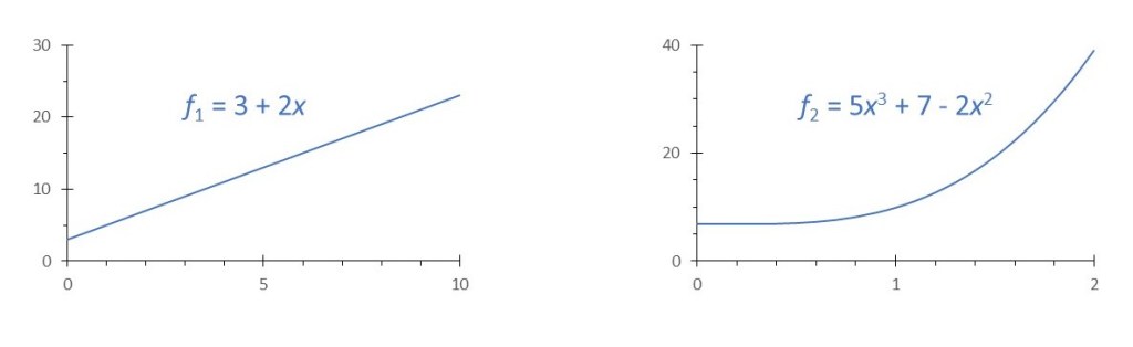
The graph of f₁ appears to be a straight line. In section 4, we see that any function of x only that has the form
f(x) = a + bx
where a and b are constants, is a straight line. In the pictures above, f₁ and f₂ have been plotted in the y-axis direction. So we can say that
y = a + bx
is the equation of a straight line.

In post 21.3 we saw that, for a circle of radius a,
x² + y² = a².
so the equation of a circle is
y =(x² – a²)^1/2.

In post 22.6, we used the equation
y = ax²
to define a parabola.

In post 22.8, we saw that the equation of a catenary is
y = acosh(x/a)
where cosh is a hyperbolic function.

So, we can see that a function of x can be represented on a graph and so defines a given type of curve. When we write y = f(x), the form of f(x) defines a curve and we say that the equation is the equation of a curve.

In polar coordinates, we define two-dimensional shapes by a radius, r, that is a function of an angle θ, as in posts 21.3 and 21.5.

4. Slope of a straight line

Let’s think about the equation   y = a + bx                    (1).

If we increase the value of x by an increment Δx, then y will increase by some amount Δy. Then equation 1 becomes   (y + Δy) = a +b(x + Δx)                    (2)

Subtracting equation 1 from equation 2 gives
Δy = a +Δx   or   Δy/Δx = a.                    (3)

The picture below shows two points, P and Q on a graph of equation 1. P has Cartesian coordinates (x, y): Q has Cartesian coordinates (x + Δx, y + Δy).

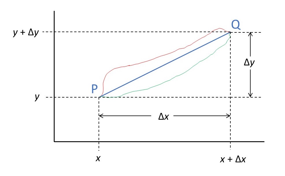
You can see that Δy/Δx is the average slope of PQ. Since Δy/Δx is a constant, whose value is a, the slope is a constant and is the shortest distance between P and Q because any curve would take a longer route, as exemplified by the red and green curves in the picture.

So, equation 1 is the equation of a straight line whose slope is a.

5. Division of zero by zero

By definition, dividing any number by itself gives the answer 1. For example, 5/5 = 1.

So you might expect that 0/0 = 1. To check whether 5/5 = 1, we can multiply both sides of this equation by 5 to give   (5/5) × 5 = 1 × 5   or   5 = 5. This result is true, so we can be confident that 5/5 = 1. Let’s do the same thing with 0/0 = 1. Multiplying both sides by zero gives 0 = 0 which is true.  But if we write 0/0 = n, where n is any number, we still get 0 = 0. So 0/0 can have any value.

Now let’s think about the value of the function (sinx)/x, where sinx is the sine of the angle x. When x = 0,. sin(x) = 0 (post 16.50). So (sin0/0) can have any value. But what happens when we make x very small and then keep making it smaller? The results are shown below (with a precision of six significant figures).

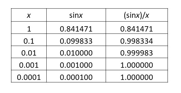
We see that, as x approaches zero, the value of our function approaches 1. We say that the limiting value of (sinx)/x, as x tends to zero, is 1. We sometimes write this statement as

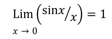
You might like to think about Xeno’s paradox (post 16.6) at this point.

6. Slope of a curve

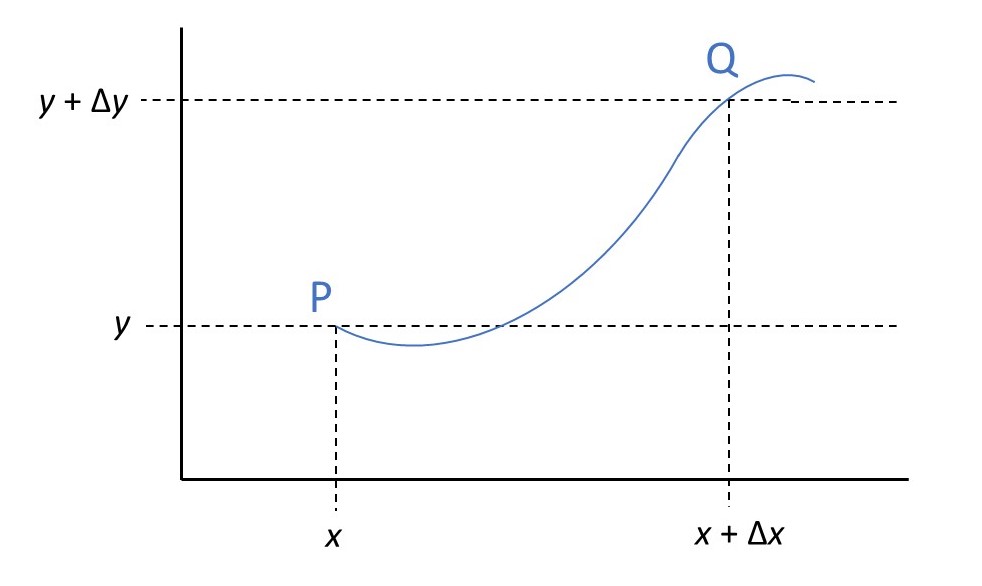
The picture above shows the graph of a function that does not represent a straight line. The average slope of the blue curve, between the points P and Q is Δy/Δx. But the slope is not the same at any point between P and Q, so this result is not very useful. If we make Δx very small, then Δy will be very small and the segment of the line is almost a straight line. In the picture, we can see that the slope of the line at R is approximately δy/δx. I am using the symbol δ, instead of Δ, to show that the increment δx is very small. The smaller the value of δx, the better the approximation.

In the limit   δx → 0,   this approximation becomes exact. We then write δy/δx as dy/dx. The process of calculating dy/dx is called differentiation and dy/dx is called the derivative of y. When we calculate dy/dx we say that we are differentiating y.

I have used Leibnitz’s nomenclature for representing the limiting value of δy/δx. This is the most commonly used. But sometimes you will see Newton’s nomenclature. He would have written the limiting value as y’. This could be confusing because it doesn’t explicitly state that the variable is x.  But this didn’t matter to Newton because, in all his calculations, the variable was time.

It might be helpful to define the derivative of f, a function of x, by the equation below.

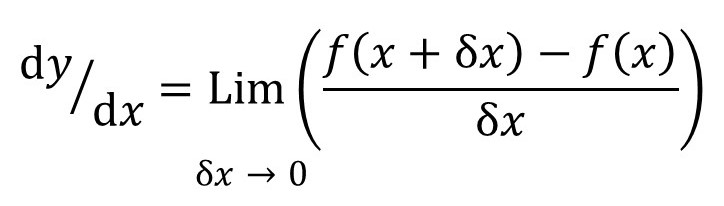
This equation defines differentiation more concisely than the explanation given above but is identical to it.

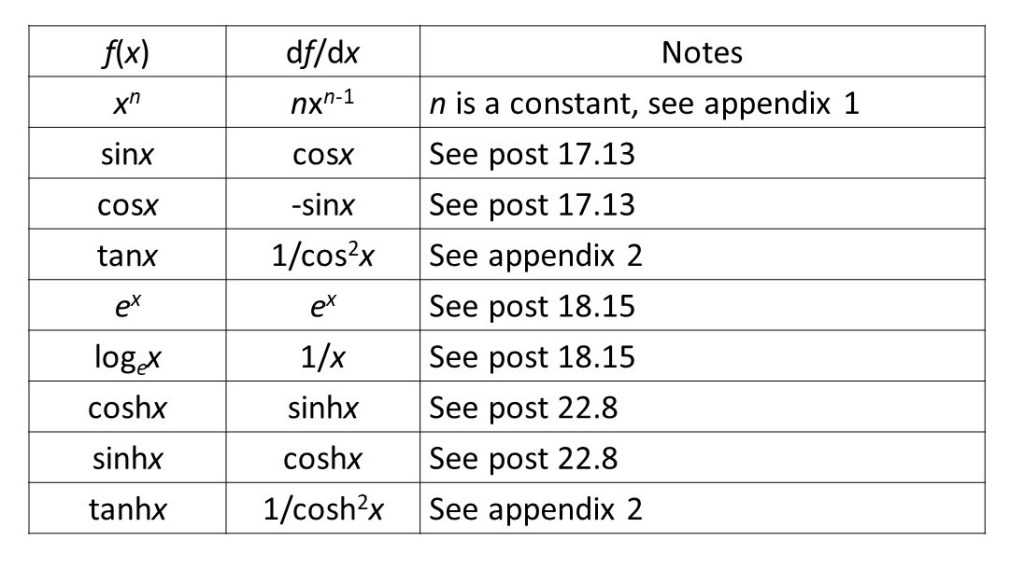
7. Derivatives of some simple functions

8. Some useful theorems

8.1 Sum of two function

If u and v are functions of x only and
f = u + v
then
df/dx = du/dx + dv/dx.
This result is proved in appendix 2.

8.2 Chain rule

If u is a function of x, the chain rule states that
df/dx = (df/du)(du/dx).
This result is justified in post 17.13.

Here is an example of how we can use the chain rule. Suppose
f = sinx² = sinu   when u = x².
Then   df/du = cosu   and   du/dx =2x.
Substituting these results into the equation that states the chain rule gives
df/dx = (cosu)(2x) = 2xcosx².

8.3 Product rule

If u and v are functions of x, the product rule states that
d(uv)/dx = u(dv/dx) + v(du/dx).

The product rule is proved in appendix 3. How do we use it? Suppose that
f= xsinx = uv   where u = x   and   v = sinx.
Then   du/dx = 1   and   dv/dx = cosx.
Substituting these results into the equation that defines the product rule gives
d(uv)/dx = xcosx +sinx.

8.4 Quotient rule

Most textbooks on calculus give the impression that we need to know the quotient rule. This isn’t true but I’ll mention it anyway.

If u and v are functions of x, the quotient rule states that
d(u/v)/dx = (1/v²){v(du/dx) – u(dv/dx)}.
We don’t need this rule, it is difficult to remember and tedious to keep looking it up. If you want to prove it, define   f = uv^-1   and   w = v^-1, then apply the product rule to differentiate.

Books may tell you that you need the quotient rule to differentiate functions like
f = (sinx)/x = uv   where   u = sinx   and   v = x^-1.
Then   du/dx = cosx   and   dv/dx = –x^-2.
We can then substitute these results into the product rule to give
df/dx = (sinx)(-x^-2) + (x^-1)(cosx) = (1/x²)(xcosx – sinx).
We didn’t need to use the quotient rule.

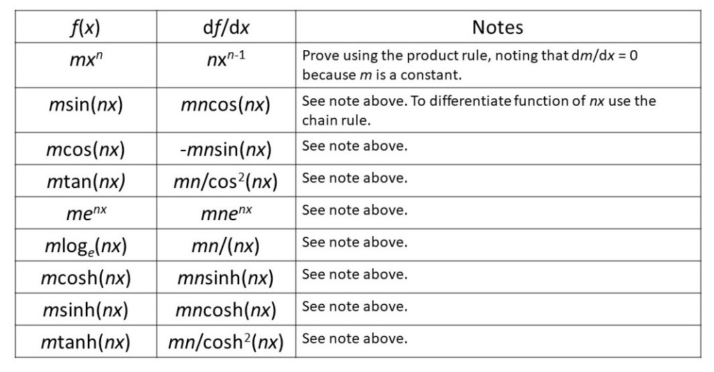
9. Derivatives of some more functions

In the table below I have made the functions of section 7 a bit more complicated. In this table n and m are constants. You can differentiate even more complicated functions using these results and the theorems in sections 8.1, 8.2 and 8.3.

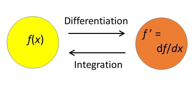
10. Integration

As explained in post 17.19, integration reverses the process of differentiation, as shown in the diagram below.

We can write that
δf = (δf/δx).δx.
So, an approximation to recovering f from (δf/δx) is given by adding together all the terms like (δf/δx).δx. We write this as

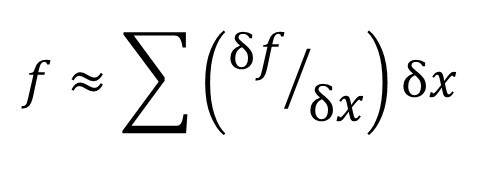
This approximation becomes exact in the limit   δx → 0   and we write the result as

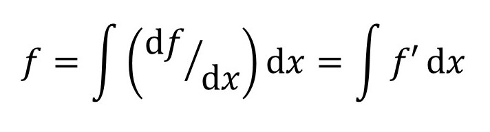
We say that f is the integral of f’. For example, since   dxⁿ/dx = nx^n-1 + C   where C is any constant, we can write that

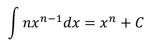
So when we perform the operation of integration a constant appears whose value is unknown. This constant, C, is called a constant of integration. When we use integration to solve physical problems, we can use boundary conditions to evaluate C, as explained in post 18.15.

So far, we have considered only indefinite integrals (see post 17.19). A definite integral is evaluated in a range of x values, for example   a ≤ x ≤ b.   Then there is no constant of integration and we can write

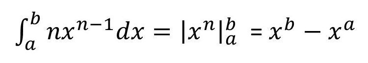
as explained in post 17.19.

The concept of a line integral is explained in post 17.36.

Examples of the application of integration are given in posts 17.19, 17.23, 17.27 and 17.36.

11. Repeated differentiation

Let’s suppose that f = x⁴.
Then we can write   f’ = df/dx =4x³.
Then we define   d²f/dx = df’/dx = 12x² = f’’
and   d³f/dx³ = df’’/dx = 24x.
Finally,   d⁴f/dx⁴ = 24   and   d⁵f/dx⁵ = 0.

12. Some applications of differentiation

Differentiation can be used to find the maximum and minimum values of a function, as described in appendix 2 of post 20.37.

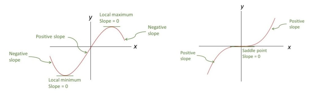
The picture above shows that a maximum, minimum and saddle point (point of inflexion) are defined by   df/dx = 0.   The three types of points are distinguished by the value of   d²f/dx²   which is negative for a maximum, positive for a minimum and zero for a saddle point.

Taylor’s theorem allows us to use the derivatives of a function to express that function as an infinite series, as described in appendix 1 of post 20.3. According to this theorem
f(x) = f(0) + xf’ + (x²/2!)f’’ + (x³/3!)f’’’ + … + (xⁿ/n!)fⁿ + …
where   n! = n × (n – 1) × (n – 2) × (n – 3) × … × 3 × 2 × 1, as described in post 18.15. For example
4! = 4 × 3 × 2 × 1 = 24.

Why is Taylor’s theorem useful? Because, for example, it allows us to derive series that represent functions like cosine (see appendix 1 of post 18.6 to see why this is useful). Also, expanding a function as a series enables us to calculate its value, for a given value of x, in the same way as we calculated the values of π (post 17.11) and e (post 18.15).

13. Partial differentiation

Suppose f is a function of more than one variable. For example, f(x, z) represents a function of x and z. An example of such a function is
f = x² + z².
We can then differentiate f with respect to x only if we assume that y is constant. To show that we are making this assumption we write the derivative as
∂f/∂x = 2x + z².
If we want it to be clear that the variable being made constant is z, we can write this as
(∂f/∂x)_z = 2x + z².
Similarly
∂f/∂z = x² + 2z.

We can differentiate the derivatives above a second time, to give
∂(∂f/∂x)/∂x = ∂²f/∂x² = 2 + z²
and
∂(∂f/∂z)/∂z = ∂²f/∂z² = x² + 2.

We can also differentiation a second time with respect to a different variable. For example
∂(∂f/∂x)/∂z = ∂²f/∂z.∂x = 2x + 2z.
Similarly
∂(∂f/∂z)/∂x = ∂²f/∂x.∂z = 2x + 2z.
Notice that the results of differentiating twice with respect to the different variables is independent of the order of differentiation. This is a general result.

Further information on partial differentiation is given in post 19.11.

14. The operator del

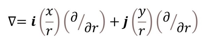
In post 20.34 we defined the operator del (also called nabla), in an orthogonal Cartesian coordinate system, by

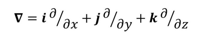
where i, j and k are unit vectors defining the directions of the axes of the coordinate system. ∇ can operate on a scalar or a vector either by forming a dot product or a cross product, as explained in post 20.34. It appears in the Navier-Stokes equation that describes fluid flow, as described in post 20.36. In post 20.37, we saw that in polar coordinates it is given, in two dimensions, by

We also saw, in post 20.34, that the scalar operator ∇² is given by

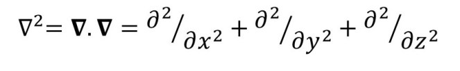
and that in polar coordinates this becomes, in two dimensions

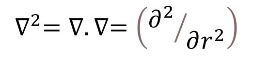
(see post 20.37). The operator ∇² appears in the wave equation (post 19.12), the diffusion equation (post 19.15) and in Schrödinger’s equation (post 19.27) which is the equation of a particle wave (see post 19.25).

15. Differential equations

Differential equations are equations that contain one or more derivatives, as described in post. An ordinary differential equation (ODE) is a differential equation that contains no partial derivatives. Examples of differential equations are the equation of a simple harmonic oscillator
d²x/dt² =-ω²x
(see post 18.11) and the equation describing exponential growth
dn/dt = kn
(see post 18.15).

A partial differential equation (PDE) contains at least one partial derivation. Examples of PDEs are the wave equation (post 19.12), the diffusion equation (post 19.15) and in Schrödinger’s equation (post 19.27).

Appendix 1

The purpose of this appendix is to show that d(xⁿ)/dx = nx^n-1.

Since x⁰ = 1 (post 18.2) is constant it does not change when x changes so
d(x⁰)/dx = 0.                    (1)

If   f = x¹ = x   then   f + δf = x + δx.   Subtracting the first equation from the second gives
δf = x   so that   δf/δx = 1.
In the limit   δx → 0   this result does not change, so that
d(x¹)/dx = 1 = x⁰ = 1x⁰.                    (2)

If   f = x²   then
f + δf = (x + δx)² = x² + (δx)² +2xδx.
The final step is explained in appendix 4 of post 17.4. Subtracting the first equation from the second gives
δf = (δx)² +2xδx   so that   δf/δx = δx +2x.

In the limit   δx → 0   this result becomes
d(x²)/dx = 2x = 2x¹.                    (3)

If   f = x³   then
f + δf = (x + δx)³ = (x + δx)(x + δx)² = (x + δx){x² + (δx)² +2xδx}.
We can write the final result as
f + δf = x{x² + (δx)² +2xδx} + (δx){x² + (δx)² +2xδx} = x³ + 3x²(δx) + 3x(δx)² +(δx)³.
Subtracting f from the left-hand side and x³ from the right-hand side gives
δf = 3x²(δx) + 3x(δx)² +(δx)³
so that   δf/δx = 3x² + 3xδx +(δx)².
In the limit   δx → 0   this result becomes
d(x³)/dx = 3x².                    (4)

We could go on to show that
d(x⁴)/dx = 4x³
d(x⁵)/dx = 5x⁴
and so on. If you want to try, it may be helpful to know that
(a + b)⁴ = a⁴ + 4a³b + 6a²b² +4ab³ + b⁴
and
(a + b)⁵ = a⁵ + 5a⁴b + 10a³b² + 10a²b³ + 5ab⁴ + b⁵.

We can already see a pattern by comparing equations 1, 2 and 3. It seems that
d(xⁿ)/dx = nx^n-1.                    (5)

The proof that follows is complicated and you may wish to trust that equation 5 is true.

If equation 4 is true then
d(x^{n + 1})/dx = (n + 1)xⁿ.                    (6)

Let’s assume that equation 5 is true and see if equation 6 follows from this assumption. If it does, we can add 1 to n when n = 1, 2, 3… and so on until we arrive at a general expression for any value of n. Then equation 4 must be true.

If n = k, we assume that
d(x^k)/dx = kx^k-1.
If equation 4 is true then
d(x^{k + 1})/dx = (k + 1)x^k.
Note that
x^{k + 1} = x(x^k)
and then differentiate this result using the product rule, the theorem stated in section 8.2 and proved in appendix 3 (below). Let   u = x   and   v = x^k. Then
du/dx = 1   and   dv/dx = kx^k-1.
The result for dv/dx rests on the assumption that equation 5 is true. The product rule states that
d(uv)/dx = u(dv/dx) + v(du/dx).
Substituting the results we have just obtained into this equation
d(x^{k + 1})/dx = x(kx^k-1) + x^k = kx^k + x^k = (k + 1)x^k.

We have shown, if equation 5 is true, then equation 6 must also be true. Therefore, we believe that equation 5 is true, as explained in the paragraph before last.

Usually we prove theorems in logical steps, starting from an axiom; this is called proof by deduction. But here we’ve used a different approach called proof by induction. In this method we prove that a statement is true when a natural number, n = 0, 1, 2, 3… has a low value. The inductive step is to show that if this statement is true when n = k, where k is a larger natural number, then it is true for n = k + 1. These steps show that the statement is true for any natural number.

A proof by deduction that   d(xⁿ)/dx = nx^n-1   is given at
 https://socratic.org/questions/differentiate-y-x-n-using-first-principle.

To understand this proof, you need to understand the binomial theorem
https://en.wikipedia.org/wiki/Binomial_theorem.

What happens when n is a fraction? Suppose n = 1/p, where p is a positive integer. Then we assume that
d(x^1/p)/dx = (1/p)x^(1/p)-1.
If this is true then
d(x^{(1/p) + 1})/dx = (1 +1/p)x^1/p.
Note that
x^{(1/p) + 1} = x.x^1/p
and continue as we did when n = k, to show that our assumption is true.

What happens when n is negative? Suppose n = – p. Then we assume that
d(x^-p)/dx = (-p)x^{-p – 1}.
If equation 4 is true then
d(x^{1 – p})/dx = (1 – p)x^-p.
Note that
x^{1 – p} = x.x^-p
and continue as we did when n = k, to show that our assumption is true.

Appendix 2

The purpose of this appendix is to show that   d(tanx)/dx = 1/cos²x   and   d(tanhx)/dx = 1/cosh²x.

In post 16.50, we defined
tanx = (sinx)/(cosx) = (sinx)(cosx)^-1 = uv
where   u = sinx   and   v = (cosx)^-1,
so that   du/dx = cosx   and   dv/dx = (sinx)/(cosx)².
To obtain the final result, we define   v = (cosx)^-1 = w^-1.
We then use the chain rule (section 8.1) to write
dv/dx = (dv/dw)(dw/dx) = (-1/w²)(-sinx) = (sinx)/(cosx)².

Putting these results into the product rule (section 8.2 with proof in appendix 3) gives
d(tanx)/dx = (sinx).(sinx)/(cosx)² + (cosx)^-1.(cosx) = (1/cos²x)(sin²x + cos²x) = 1/cos²x.
The final step is true because   sin²x + cos²x = 1 (post 16.50).

You will usually see this result written as sec²x. The trigonometric secant is defined by secx = 1/cosx. Similarly, cosecant is defined by cosecx = 1/sinx. I never use them because I can’t remember which is which. I don’t believe anyone really needs them.

Appendix 3

The purpose of this appendix is to prove the theorem of section 8.1. If   f = u + v,
where f, u and v are functions of x,
then   f + δf = u(x + δx) + v(x + δx).
Subtracting the first equation from the second gives
δf = u(x + δx) + v(x + δx) – u – v.
Dividing by δx gives

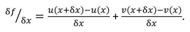
Notice that, in the limit   δx → 0   the right hand side of this equation becomes du/dx + dv/dx   and the left hand side is df/dx (see section 6), which proves the theorem.

Appendix 4

The purpose of this appendix is to prove the theorem of section 8.3.

If   f = uv,
where f, u and v are functions of x,
then   f + δf = (u + δu)(v + δv) = uv + uδv + vδu + δu.δv.
Subtracting the first equation from the second gives
δf = uδv + vδu + δu.δv.
Dividing by δx gives
δf/δx = u(δv/δx) + v(δu/δx) + (δu.δv)/δx.
In the limit   δx → 0   this becomes
df/dx = u(dv/dx) + v(du/dx)
since   δu.δv   represents two infinitesimally small numbers multiplied by each other.