Before you read this, I suggest you read posts 20.34 and 20.36.

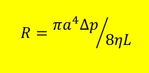
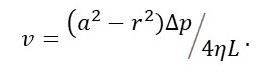
Poiseuille’s equation (highlighted in yellow above) enables us to calculate the rate of flow, R (volume divided by time), of a liquid of viscosity Ƞ in a narrow horizontal tube of radius a and length L, when there is a pressure difference, Δp, between its ends. It is named after the French physicist Jean Poiseuille (1797-1869). We derived an equation of this form in post 17.42, using dimensional analysis. But this method does not tell us that a constant (1/8) is involved and we couldn’t be certain that the equation didn’t involve trigonometric or exponential terms that are dimensionless.

In this post we will see how Poiseuille’s equation can be derived from the Navier-Stokes equation (post 20.36). There are easier ways of deriving Poiseuille’s equation but the method used here demonstrates how we can use the Navier-Stokes equation to solve a problem. This is not an easy subject to understand and is the last of four posts (the others are 20.34, 20.35 and 20.36) about the Navier-Stokes equation. If you are not very interested in the mathematics of fluid flow, it might be better to read post 17.15, to find out about the Navier-Stokes equation, and post 17.42, to find out about Poiseuille’s equation (although it would be useful to look at appendix 3, below) and not read this posts 20.34, 20.35 or20.36.

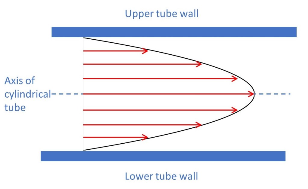
When a fluid flows in a tube, the flowing liquid is in contact with a solid surface. At the interface between the solid and liquid, there is a layer in which the liquid is stationary, called the boundary layer. What is the evidence for the boundary layer? Many books are evasive about this question or simply state that it can be observed experimentally. I think the experimental evidence is weak – it would be difficult to detect an infinitesimal layer of liquid that wasn’t moving. I believe that the best evidence for the boundary layer is that, if we assume that it exists, it enables us to make predictions that fit our observations about fluid flow.

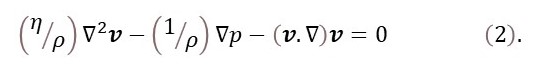
We will start our derivation with the Navier-Stokes equation for incompressible flow (posts 20.35 and 20.36) which states that

The operators ∇² and ∇ are defined in post 20.34. The fluid, of density ρ, flows with a velocity v as a result of the pressure difference between the ends of the tube and a potential function Ψ (post 20 36); the pressure, p, varies long the length of the tube because the flow leads to a drop in pressure. If the potential energy of the fluid is purely gravitational, Ψ = gh, where g is the magnitude of the gravitational field, and h is difference in height between the ends of the tube (post 20.36). The first term on the right-hand side of the equation is the partial derivative (post 19.11) of the modulus of v with respect to time, t. In this post all the symbols written in bold are vectors; the others are scalars (post 17.3).

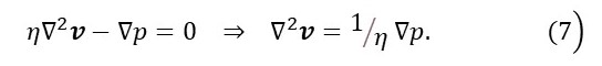
Since Poiseuille’s equation applies only to laminar flow, the partial derivative of v with respect to t is zero (post 20.36). If the only potential energy is gravitational, for a horizontal tube (whose ends both have the same height) Ψ = 0. Then we can simplify equation 1 to

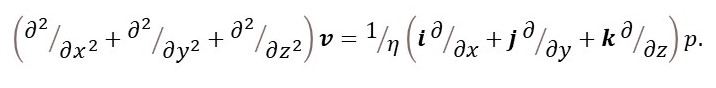
We will use the axis of the tube to define the z-axis of an orthogonal Cartesian coordinate system (post 16.50). Then we can write

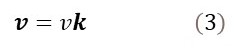
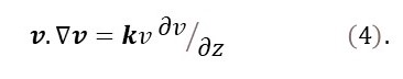
where k is a unit vector in the z-axis direction (post 17.3). Be careful! Although the flow is in the z-direction, its magnitude can still change perpendicular to the flow direction. In post 20.36, we saw equation 3 means that

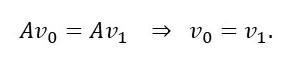
Let’s suppose that the speed of the liquid at the beginning of the tube is v₀ and at the end of the tube is v₁. The tube has a constant cross-sectional area A. If we now apply the continuity equation (post 17.15)

We could apply this argument to any two points along the tube to conclude that v doesn’t change as z changes. Then

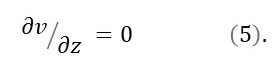
From equations 4 and 5

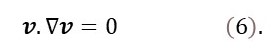
Notice that this isn’t always true because a liquid could flow through a channel whose cross-sectional area isn’t constant – so we couldn’t use equation 6 in post 20.36. But, for a tube with a constant radius, A is constant, so equation 6 is true.

Substituting the result from equation 6 into equation 2, and multiplying both sides of the equation by ρ gives

We can write this result (see post 20.34) as

Noting equations 3 and 5, the left-hand side simplifies to

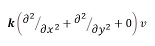
and, since the pressure difference acts along the axis of the tube only, the right-hand side simplifies to

So we can write equation 7 as

The moduli of both sides of this equation must be equal, so that

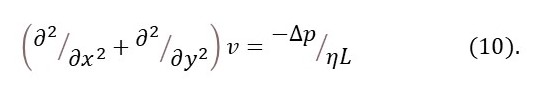
If we assume that a graph of v against x or y is a smooth curve, both the second derivatives on the left-hand side of this equation will be constant. Then

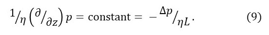
Now equation 7 becomes

The minus sign in equation 10 arises because p decreases as L increases since the flow causes the pressure to drop. We could continue to describe any point within the tube, at a given value of z, by the values of x and y. But we can use the symmetry of the tube to simplify the mathematics if we replace x and y by a radial distance, r, from the axis of the tube. According to Pythagoras’ theorem (post 16.50, appendix 1)

Now we can write equation 10 in the form

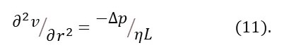
Further details of this step are given in appendix 2.

Integrating (post 17.19) equation 11 with respect to r gives

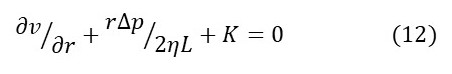
where K is the sum of the constants of integration (post 17.19). To find K we apply the boundary condition

How do we know this? The reason is that a graph of v plotted against r must have a maximum value at r = 0 because v decreases, as r increases (in any direction), to a value of 0 at the tube-liquid interface (the boundary layer). If you don’t know about the values of derivatives when functions pass through maxima and minima, see appendix 2 to help you understand this explanation.

Appling this boundary condition to equation 12 shows that K = 0 so that equation 12 becomes

Integrating again with respect to r gives the result that

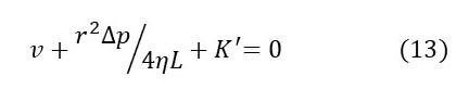
where K’ is another sum of constants of integration. To find K’, we note that in the boundary layer (r = a), v = 0. So, from equation 13,

Substituting this value for K’ into equation 13 gives the result that

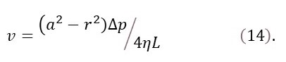
Equation 14 provides some interesting results about how the speed of the flowing liquid depends on r. This is discussed in appendix 3. I have put this in an appendix because I don’t want to disrupt the derivation of Poiseuille’s equation. But, after you have finished reading about this derivation, I suggest you read appendix 3.

We have already noted that the value of v decreases from its maximum value (when r = 0) to zero (when r = a).

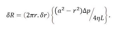
So, to determine the total flow rate, we will first consider the flow perpendicular to an annulus, of infinitesimal thickness δr, as shown in the picture above. Since the annulus is in the plane of the tube cross-section, it is perpendicular to the flow direction z. The rate of flow is given by the rate of change of volume, that is by the area of the annulus (its thickness multiplied by its circumference, since δr is infinitesimally small) multiplied by the speed of flow. So, from equation 14

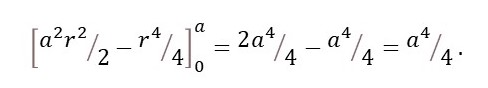
Integrating this result between the limits r = 0 and r = a (post 17.19) gives

since integrating δR with respect to r consists of adding the flow across all the infinitesimal elements. all the infinitesimal elements. (If this isn’t clear, see post 17.19).

Substituting this result into the right-hand side of equation 15 gives Poiseuille’s equation – in case you’ve forgotten, the equation highlighted in yellow at the beginning of this post.

If you’ve read this to the end – well done! You will have realised that using the Navier-Stokes equation to solve even very simple problems is not easy. So, you will now understand why computational fluid dynamics (post 20.36) is so useful.

Related posts

17.15 Fluid flow
20.35 Incompressible and compressible fluid flow
20.36 The Navier-Stokes equation

Appendix 1

The purpose of this post is to show that

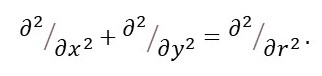
Note that this result is only true for a cylindrically symmetric system that is not accelerating in the z-direction.

The position of the point P, in the picture above, can be specified by the orthogonal Cartesian coordinates (origin at O, post 16.50 appendix 1) x and y or by the radial distance, r, and the angle θ; (between OP and the x-axis); r and θ are called polar coordinates.

We have already seen that

Differentiating equation A1 with respect to x gives

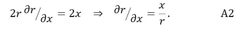
Similarly

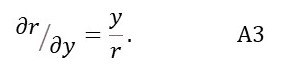
Now

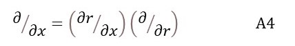
as explained in the appendix to post 19.12. From equations A2 and A4

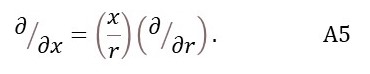
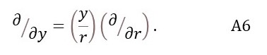
Similarly

Since there is no acceleration in the z-direction, by definition (see post 20.34)

Substituting the partial derivatives from equations A5 and A6

From equations A1 and A8

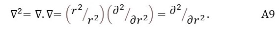
Comparing equations A7 and A9 gives the required result.

Appendix 2

The purpose of this appendix is to show that the derivative of a function is zero when it passes through a maximum or a minimum.

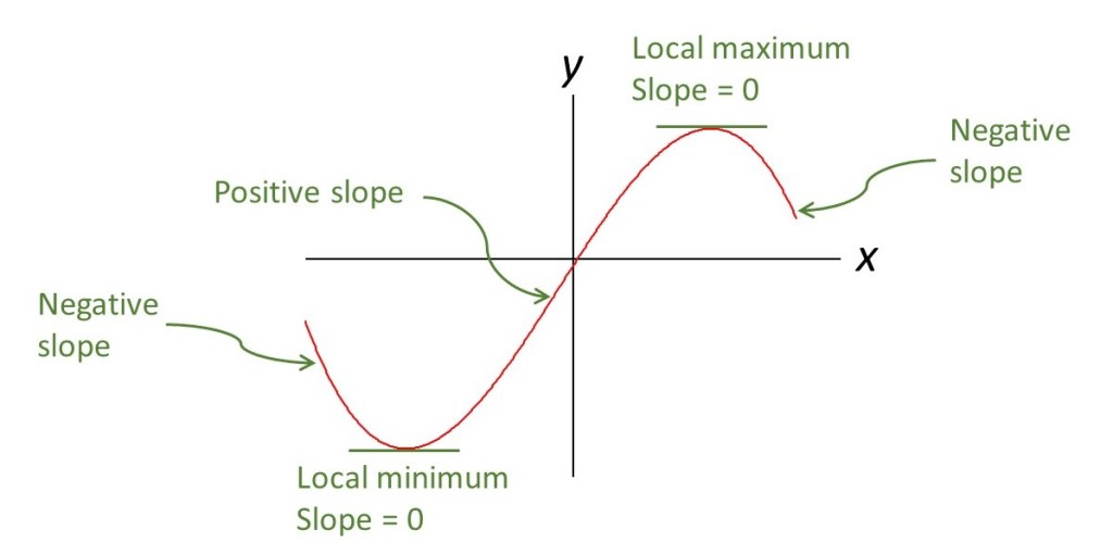
The picture above shows y (a function of x) plotted against x. The curve passes through a local minimum, where the slope changes from negative to positive. At this point, the slope dy/dx = 0. It also passes through a local maximum, where the slope changes from positive to negative. At this point, the slope is also given by dy/dx = 0.

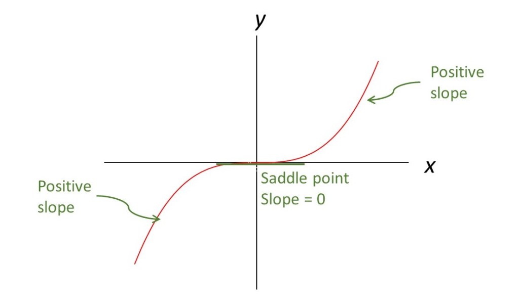
The picture above shows y (now a different function of x) plotted against x. The curve has a point of zero slope (dy/dx = 0) between two positive slopes. This point is neither a maximum nor a minimum and is called a saddle point or a point of inflexion.

But note that, for a minimum, the slope dy/dx changes from negative to positive so that d²y/dx² is positive. For a maximum, the slope dy/dx changes from positive to negative so that d²y/dx² is negative. And for a saddle point, the slope the slope dy/dx doesn’t change so that d²y/dx² is zero.

In case this is completely new to you, I am going to give an example of how to use these ideas.

The picture above shows a square sheet of cardboard of side a. We want to cut along the corner squares, as shown, and fold along the red dotted lines to make a box. We also want the box to have the maximum possible volume. What should be the length we cut along the corner squares, to achieve this result?

Let x represent the length of the cuts. Then the base of the box will be a square of side (a – x), so its area will be (a – x)². The height of the box will be x and its volume (the area of the base multiplied by the height) is

Differentiating this result gives

The condition that dV/dx is zero is met either by

The first solution (the x = a/2) gives a box with zero volume; this is the minimum value possible for the volume of the box. Then the other solution appears to be the one that we want.

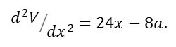
How can we be sure this gives us a maximum value of V? We differentiate equation B1 to give

Now we substitute the second possible value of x from equation B2 into this result to get

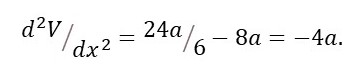
Since a must be positive (it’s the side of a square of cardboard), d²V/dx² is negative, so the second solution (x = a/6) gives us the maximum value for V.

Appendix 3

The purpose of this appendix is to explore what equation 14 tells us about the speed of flow at different values of r within the tube.

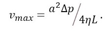
The equation above is a copy of equation 14. Then v must have its maximum value, v_max, when r = 0; the same result was obtained in the main text. As a result

In the graph below, I have plotted r against v. To plot this graph I have arbitrarily assigned values of a = 1 unit and Δp/(4ηL) = 1unit.

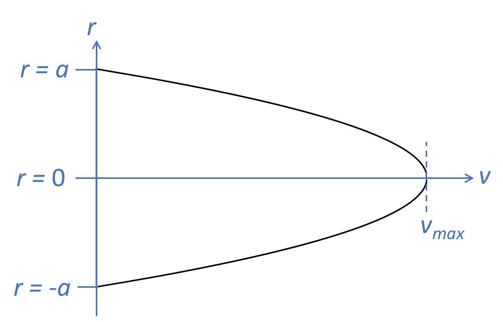
We can see that the graph is the shape of a parabola; v has its maximum value when r = 0 and falls to zero when r = a. In the picture below, this graph is translated into a picture of the speed of flow within the tube, where the red arrows represent the velocity vectors, at selected values of r, whose envelope is described by the parabola.