To understand this post you need to be familiar with the contents of post 18.2.

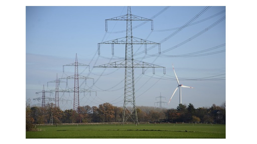
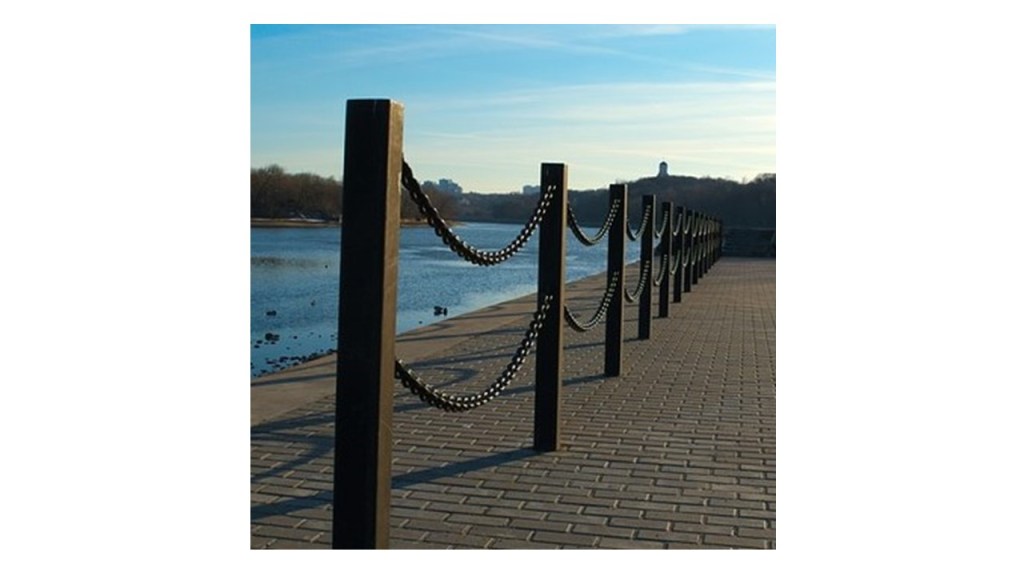
The picture above shows cables supported by pylons; each section of cable hangs from two fixed points. Between these points, the force of gravity stretches the cable so that it falls into a curve. Until the early seventeenth century, people believed this curve was a parabola. Why? Because it looked like one! But Galileo Galilei (1564-1642; known for the Galilean principle of relativity and describing the motion of planets relative to the sun, see post 16.9) doubted that this assumption was true. In 1691, the equation that really describes the curve was derived by Christiaan Huygens (1629-1695), Gottfried Leibnitz (1646-1716) and Johann Bernoulli (1667-1748). Huygens was a Dutch mathematician, responsible for Huygens’ principle. Leibnitz was a German philosopher and mathematician who thought of differentiation and integration independently of Newton, and at about the same time. Bernoulli was a Swiss mathematician, the father of Daniel Bernoulli who derived Bernoulli’s equation. We call the curve whose equation they derived the catenary. The word “catenary” comes from the Latin word catena meaning a chain because the smooth curve through the centroid of each link of a chain, supported at two ends, lies on a catenary – see the picture below.

In appendix 1, I show that the equation of the catenary is

y = a(e^x/a + e^-x/a)/2                    (1)

where the number e has an approximate value of 2.718 and a is a constant. Here x and y are the horizontal and vertical axes (respectively) of a right-handed Cartesian coordinate system. The lowest point on the curve (the minimum of the catenary) is defined to have x=0. We’ll think about the definition of the zero value of y later. Equation 1 is usually written as

y = acosh(x/a).                    (2)

Here cosh is an example of a hyperbolic function defined by

coshx = (e^x + e^-x)/2.

More details are given in appendix 2.

The minimum value of the catenary was defined to have x = 0. Substituting this value into equation 1 gives a minimum value for y of

y_min = a(e^0/a + e^-0/a)/2 = a(e⁰ + e^-0)/2 = a(1 + 1) = a.                    (3)

If you’re not sure why e⁰ = 1, see post 18.2. When a = 0, y_min = 0. The origin of our coordinate system is now defined because we have already defined the minimum of the catenary to have x = 0. So when a > 0, y_min is positive.

Let’s apply equation 1 to a cable of uniform cross-sectional area A that is made of a material with a density ρ. Then appendix 1 shows that

a = T₀/(ρgA).                    (4)

Here T₀ is the modulus of the tension in the cable when x = 0, defined to be its lowest point; g is the modulus of the gravitational field acting on the cable. From equations 3 and 4

y_min = T₀/(ρgA).                    (5)

Since y_min is positive, equation 5 shows that the cable drops lower (lower value of y_min) when its tension is reduced, which is what we would expect. It also shows that the cable will drop lower when ρ and A are increased. This is also what we would expect because increasing ρ and A increases the mass of the cable and, hence, the gravitational force pulling it downwards. The picture below shows the shape of the catenary, for different values of a, plotted using equation 1.

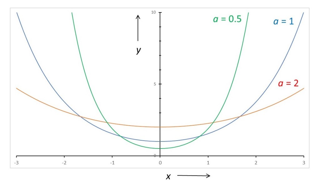
You can see that the shape of the curves looks a lot like the shape of a parabola (see post 22.6). But it’s not the same because the value of y is never zero, for non-zero values of a. This should warn us that, just because an object appears to have a geometric shape that we know about, the appearance can be deceptive!

Related posts

22.7 The caustic curve
21.5 Logarithmic spirals
21.3 Polar coordinates, circles and spirals
17.40 Rolling

Appendix 1

The purpose of this appendix is to derive equations 1 and 2.

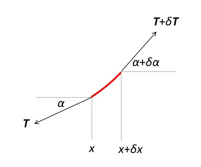
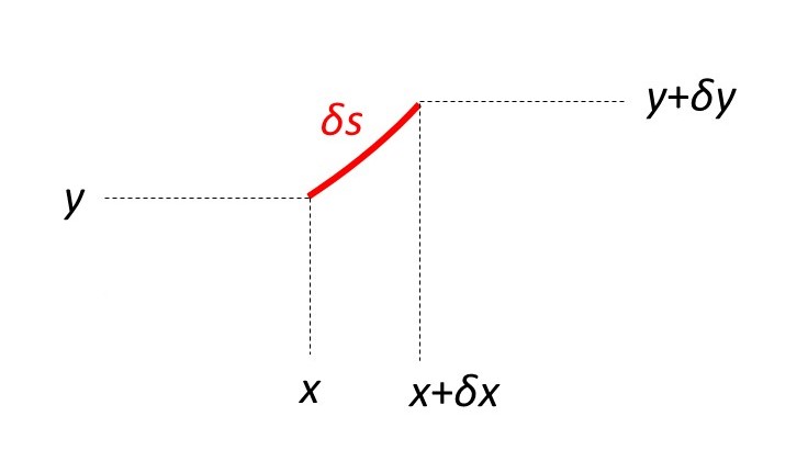
In the picture above, the red line is an infinitesimal length, δs, of a catenary between x and x + δx. At the lower point (x-coordinate x), the tension in the cable is the vector T. Since, at the higher point (x-coordinate x + δx), the cable supports the weight of the cable below, the tension is greater than at the lower point and is represented by T + δT. I define the angle that the red element makes with the horizontal (x-axis direction) as α (at x) and α + δα (at x + δx).

I am now going to consider the forces acting on the element in the horizontal (x-axis) direction. Then

-(Tcosα)i + {(T + δT)cos(α + δα)}i = 0.

Here i is a unit vector in the x-axis direction. For this result to be true

Tcosα = (T + δT)cos(α + δα)

which is another way of saying that Tcosα is constant. Then we can define the constant T₀ by

T₀ = Tcosα.                    (A1)

Another way to think about T₀ is that, at the lowest point of the catenary, α = 0; so all the tension is in the horizontal direction. Also, since cos0 = 1, the modulus of this tension is equal to T₀. Then T₀ is the modulus of the tension in the cable at its lowest point that defines (main text) x = 0.

I am now going to consider the forces acting on the element in the vertical (y-axis) direction. Then

-(Tsinα)j + {(T + δT)sin(α + δα)}j – jδF= 0.

Here j is a unit vector in the x-axis direction and δF is the modulus of the gravitational force acting on the element. From this result, we see that

–Tsinα + Tsin(α + δα) + (δT)sin(α + δα) = δF.                   (A2)

Now we use the expression for the sine of sum of angles to give

sin(α + δα) = (sinα)(cosδα) + (cos α)(sinδα) ≈ sinα.

The final step arises because δα is infinitesimal and because sin0 = 0 and cos0 = 1. We can combine this approximation in equation A2 to give

(δT)sinα ≈ δF.

Since T is a constant, for a given value of x, we can write

δ(Tsinα) ≈ δF.

Substituting for T, from equation A1, gives

δ(T₀sinα/cosα) ≈ δF   or   δ(T₀tanα) ≈ δF.

But tanα is the slope of the curve dy/dx, so that

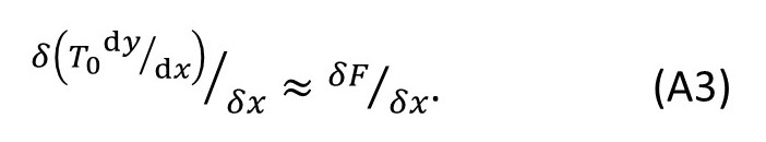
δ(T₀.dy/dx) ≈ δF.

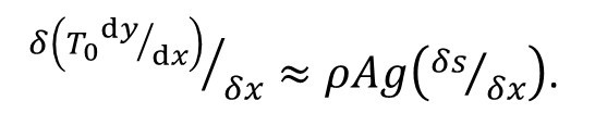
Dividing both sides of this result by δx gives

If δm is the mass of the element, then

δF = gδm = ρAgδs

where g, ρ and A are defined in the main text. Therefore

δF/δx = gδm = ρAg(δs/δx).

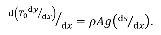
Then equation A3 becomes

In the limit δx → 0, the approximation becomes exact with the result that

Now I’m going to use the result for ds/dx, from appendix 3, in this result, to give

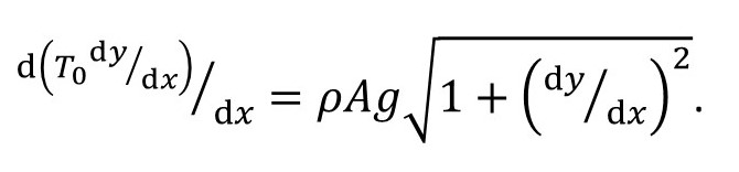
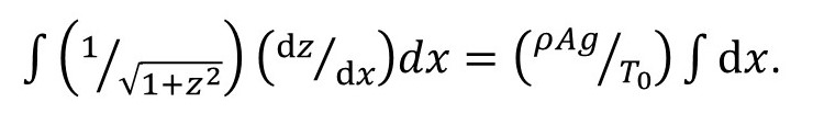
This equation looks horrendous! What can we do with it? We can define z = dy/dx so that it can be written

T₀(dz/dx) = ρAg(1 + z²)^1/2

noting that T₀ is a constant. (In these appendices I use a square root sign or raise something to the power ½, which are the same, depending on whichever is the easiest to type – that’s the only reason). Rearranging this result gives

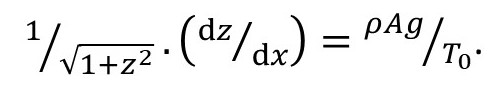
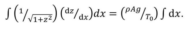
Integrating with respect to x gives

To make everything look neater, I note that T₀/ρAg is a constant that I’m going to call a. Making this substitution, and simplifying the left-hand side gives

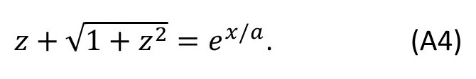
 Evaluating these integrals (see appendix 4) gives

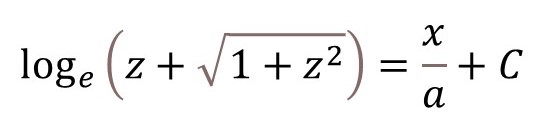
where C is a constant of integration. Remember that z = dy/dx and that at x = 0, the curve is at its lowest point (a minimum) so that dy/dx = 0. Using this information as a boundary condition, we see that

0 = 0 + C   or   C = 0.

Then the result above becomes

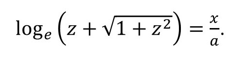
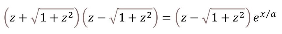
From the definition of a logarithm to the base e, this can be written as

Multiplying both sides by z – (1 + z²)^1/2 gives

which gives

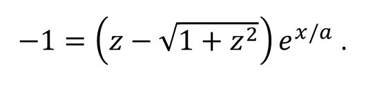
I explain the last step in appendix 5 in case this is difficult to follow.  Multiplying both sides by e^-x/a gives

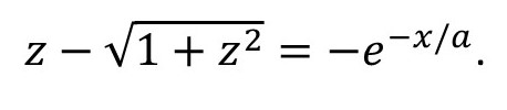
Adding this result to equation A4 gives

2z = e^x/a – e^-x/a.

Remember that z = dy/dx, giving

2(dy/dx) = e^x/a – e^-x/a.

Integrating with respect to x gives

y = B + a(e^x/a + e^-x/a)/2

where B is a constant of integration. The effect of changing the value of B is to add to, or subtract from, the value of y which means it moves the position of the origin of our coordinate system. Since we haven’t defined the position of the origin (except in the x-axis direction) in this appendix, I shall define B to be equal to zero. The consequence of this decision is described in the main text. Then

y = a(e^x/a + e^-x/a)/2 = acosh(x/a)

where the hyperbolic function cosh is discussed in appendix 2. This result is presented as equations 1 and 2 in the main text.

If you’ve managed to follow this to the end – congratulations!

Appendix 2

The purpose of this appendix is to introduce the hyperbolic functions sinh and cosh.

According to Euler’s relation

e^iθ = cosθ + isinθ

where i is the square root of -1 (see post 18.6). Since cos(-θ) = cosθ and the sin(-θ) = -sinθ (see post 16.50), it follows that

e^-iθ = cosθ – isinθ.

Adding these two equations gives

cosθ = (e^iθ + e^-iθ)/2.

Subtracting one from the others gives

sinθ = (e^iθ – e^-iθ)/2.

By analogy, we define the hyperbolic functions, by omitting i to give

coshθ = (e^θ + e^–θ)/2   and   sinhθ = (e^θ – e^–θ)/2.

It follows from these definitions that

d(coshθ)/dθ = sinhθ   and   d(sinhθ)/dθ = coshθ,

also that

cosh²θ + sinh²θ = 1.

By analogy with the tangent of an angle, we define

tanhθ = sinhθ/ coshθ.

Appendix 3

The purpose of this appendix is to introduce the concept of the length of a curve.

The picture above shows an infinitessimal length, δs, of curve between the points (x, y) and (x + δx, y + δy). Since δs is infinitesimal, it is almost a straight line. Applying Pythagoras’ theorem gives

(δs)² ≈ (δx)² + (δy)².

Dividing both sides by (δx)² gives

(δs)²/(δx)² ≈ 1 + (δy)²/(δx)².

In the limit δx → 0, this approximation becomes exact (see post 17.4) with the result that

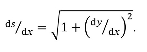
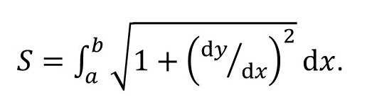
Then the length, S, of a curve in the range a < x < b is defined by the definite integral

Appendix 4

The purpose of this equation is to consider the indefinite integral

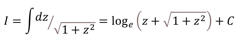
where C is a constant of integration. To evaluate the integral, I consulted the table of standard integrals at https://www.maths.usyd.edu.au/u/UG/JM/MATH1003/r/m1003/Table_of_Integrals.pdf.

I checked this result by differentiating the right-hand expression for I with respect to z (see post 17.19).

First, I define

so that

I = log_eu + C.

Differentiating I with respect to u (see post 18.15) gives

dI/du = 1/u.

du/dz = 1 + (1/2)(1 + z²)^-1/2(2z) = 1 + {z/(1 + z²)^-1/2}.

Note that

1 + {z/(1 + z²)^-1/2 = {(1 + z²)^1/2 + z}/(1 + z²)^1/2 = u/(1 + z²)^1/2.

Also note that (see appendix 1.2 of post 17.13)

dI/dz = (dI/du)(du/dz) = (1/u){ u/(1 + z²)^1/2} = 1/(1 + z²)^1/2.

So the result of evaluating the integral, at the beginning of this appendix, is true.

Appendix 5

The purpose of this appendix is to remove some tedious algebra from appendix 1.