Before you read this, I suggest that you read posts 17.4 and 18.10.
In post 18.10 we saw that a one-dimensional wave could be represented by a wave function, ψ, that is a function (post 19.10) of position, x, and time, t. At a fixed point in space (x is constant), the wave function is given by
ψ = Asin(2πt/T) = Asin(2πft) = Asin(ωt). (1)
At a fixed time
ψ = Asin(2πx/λ) = Asin(2πkx) = Asin(κx). (2)
In equations 1 and 2, A represents the amplitude of the wave whose time period (post 18.10) is T and whose wavelength (post 18.10) is λ.
We can find the rate of change of ψ by differentiating (post 17.4) equation 1 with respect to time. We can perform an analogous operation in space by differentiating equation 2 with respect to x. But, when we differentiate equation 1, we are assuming that x is constant. And, when we differentiate equation 2, we are assuming that t is constant.
When we differentiate something that is a function of more than one variable, by assuming that all but one of the variables is a constant, the operation is called partial differentiation. To show that the result is a partial derivative we replace the usual d that appears in differentiation by ∂ (we call this symbol “partial d”).
Using the result for differentiating sines from appendix 1.1 of post 17.13 gives
∂ψ/∂t = ωAcos(ωt) and ∂ψ/∂x = κAcos(κx).
That was easy because we started with an expression for ψ when x is constant and an expression for ψ when t is constant (equation 2).
Usually we want to perform partial differentiation when our starting equation contains three or more variables. For example, let’s think about the volume, V, of an ideal gas (post 18.25) containing n moles (post 17.48) at a pressure p and temperature (on the Kelvin scale, post 16.34), T. Be careful – I’m now using T to represent something completely different in the second part of this post. Normally, I would avoid doing this but T is so commonly used to represent the time period of a wave and temperature on the Kelvin scale, that I’ve used it to represent both. According to the ideal gas equation (post 18.25)
V = nRT/p = nRTp-1 (1)
We can calculate the effect on V of changing T by assuming that p is constant and calculating
∂V/∂T = nRp-1 = nR/p. (2)
We can calculate the second partial derivative (post 17.4) of V with respect to T as
∂2V/∂T2 = 0 (3)
since, in this operation, we are assuming that p is constant. If you’re not sure about how equations 2 and 3 were calculated, see post 17.4.
Similarly, we can calculate the effect on V of changing p by assuming that T is constant and calculating
∂V/∂p = –nRTp-2 = –nRT/p2. (4)
And we can calculate the second partial derivative (post 17.4) of V with respect to p as
∂2V/∂p2 = nRTp-3 = nRT/p3. (5)
If you’re not sure about how equations 4 and 5 were calculated, see post 17.4.
We can also calculate:
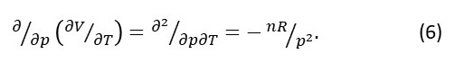
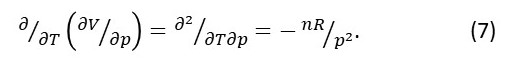
Notice that equations 6 and 7 give the same results.
The ideas developed here will be useful when we use differential equations (post 19.10) to describe things that depend on time and space – like diffusion (post 18.26) and wave motion (post 18.10).
Related posts
19.10 Differential equations
18.17 Euler’s relation, oscillations and waves
18.16 The square root of minus 1 and complex numbers
18.15 More about exponential growth: the number e
18.14 Wave shapes – Fourier series
18.3 Logarithms
17.37 More about torque – cross products of vectors
17.36 More about work – line integrals
17.19 Calculating distances from speeds – integration
17.4 Displacement, velocity and acceleration
17.3 Three-dimensional vectors
Follow-up posts
