Before you read this, I suggest you read post 19.14.

In post 19.12, we saw how a wave could be represented, in time and space, by the wave equation.

The concentration of a diffusing substance also varies in both space and time (post 18.26). Can we represent this dependence by a differential equation too? In post 19.14, we saw how conduction of heat behaves like diffusion – so the differential equation that describes diffusion should also describe conduction.

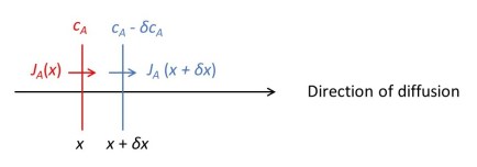
The picture above shows a section through a red and blue surface each with a unit area – as in the figure of post 19.14. The two surfaces are an infinitesimal distance, δx, apart and diffusion of a substance A occurs in the direction shown by the arrow. The concentration of A at the red surface is c_A and at the blue surface c_A – δc_A, as described in post 19.14. But now we are going to consider the rate of flow of A across each surface; it will be less across the blue surface than across the red surface, because the concentration is less. If the rate of flow across the red surface is J_A(x), then the rate of flow across the blue surface will be J_A(x + δx); here J_A is not multiplied by whatever is in the brackets – the brackets denote that J_A is a function of whatever is in the brackets, as described in post 19.10.

The rate at which the number of particles of A is increasing, between the red and blue surfaces, is J_A(x) – J_A(x + δx). We can also express this result as the rate at which the concentration (number of particles per unit volume) between the surfaces is increasing, multiplied by the volume between the two surfaces. The rate of increase of concentration is the derivative of c_A with respect to time (post 17.4), ∂c_A/∂t; this is a partial derivative because c_A depends on both x and time, t (post 19.11). Since the two surfaces have unit area, the volume between them is δx. Therefore, we can write that

(∂c_A/∂t)δx = J_A(x) – J_A(x + δx).                    (1)

Since δx is infinitesimally small, we can write

J_A(x + δx) – J_A(x) ≈ (∂J_A/∂x)δx.                    (2)

This result is obtained by noting that J_A(x + δx) – J_A(x) = δJ_A = (δJ_A/δx)δx.

From equations 1 and 2

∂c_A/∂t = -(∂J_A/∂x).                     (3)

According to Fick’s law (post 19.14)

J_A = D_AB(∂c_A/∂x)

where D_AB is the diffusion constant for A in a medium B (post 19.14). Substituting this definition of J_A into equation 3 gives

The final step arises because D_AB is a constant.

The result, that

is called the one-dimensional diffusion equation or Fick’s second law. You might like to compare it with the one-dimensional wave equation of post 19.12.

In post 19.14 we saw that conduction of heat was analogous to diffusion and was described by Fourier’s law

J_Q = – k(dT/dx)                    (5)

where J_Q is the rate of flow of heat, across unit area perpendicular to the direction of flow, dT/dx is the temperature gradient and the constant, k, is the thermal conductivity of the substance the heat is flowing through.

We can derive an equation, analogous to equation 4, to describe the distribution of temperature in an object that is conducting heat. To do this, we need to relate heat (post 16.35) and temperature (post 16.34). The specific heat capacity, C, of mass m of a substance is defined by

C = (1/m)(ΔQ/ΔT)

where ΔT is the increase in temperature required to increase the heat in the substance by ΔQ. This result can be written as

ΔQ = mCΔT.

What is the total quantity of heat in a sample of a substance at temperature T? If we measure T in degrees Kelvin, there is no heat when T = 0 K (posts 16.34 and 16.35). (K is the abbreviation for “degrees Kelvin). When we increase the temperature to T, the heat in the sample is

Q = mCT

so that

dQ/dt =mC(dT/dt).

If we follow the derivation of equation 4 from Fick’s law, but now consider the flow of heat between the red and blue surfaces, equation 1 becomes

mC(∂T/∂t)δx = J_Q(x) – J_Q(x + δx)

with the result that

where h is called the thermal diffusivity of the substance.

Now let’s think about three-dimensional diffusion of A in B. If B is isotropic, that is if its properties are the same in all direction, equation 4 becomes

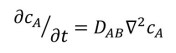
where the inverted triangle represents the Laplacian operator, defined in post 19.12. If the properties of B are anisotropic, that is if its properties are not the same in different directions, than  is not a single number; it’s value depends on direction – so  it’s not a scalar (post 17.2). But it isn’t a vector (post 17.2) either because its value in one direction isn’t independent of its value in a perpendicular direction – because diffusion in one direction depletes the pool of molecules available to diffuse in a perpendicular direction. Then D_AB is a tensor – I hope to write more about tensors in a much later post.

So, what do the solutions of the diffusion equation (equation 4) look like? They must represent a concentration that becomes more evenly distributed as time passes – as explained in post. I will demonstrate this mathematically in the next post.

Related posts

19.14 Fick’s law
19.12 The wave equation
19.11 Partial differentiation
19.10 Differential equations
18.27 Diffusion through membranes
18.26 Diffusion
16.35 Heat
16.34 Temperature