Before you read this, I suggest you read post 22.4.

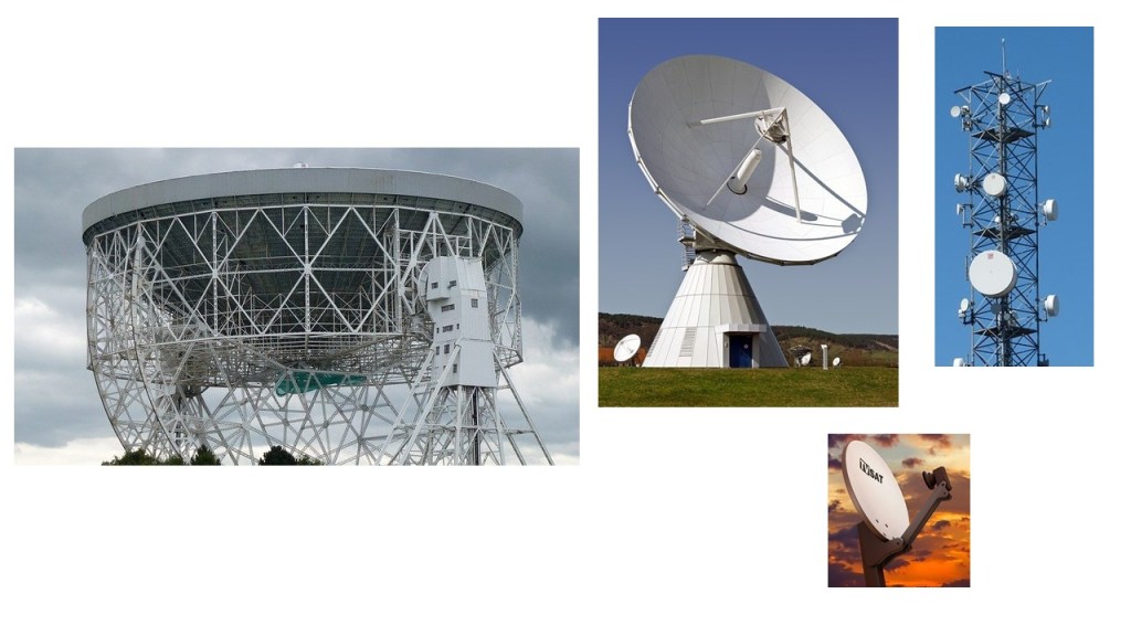
When I wrote about reflection in post 22.4, I concentrated on reflection of light by a mirror. Concave mirrors are useful but the more familiar applications of reflection at concave surfaces involve focussing radio waves and microwaves from distant objects. Examples include radio-telescopes, receivers for Radar, mobile phone masts and the satellite dishes used for television reception. In all these examples, the source is so far from the receiver that all rays from the source can be considered parallel (see post 22.1).

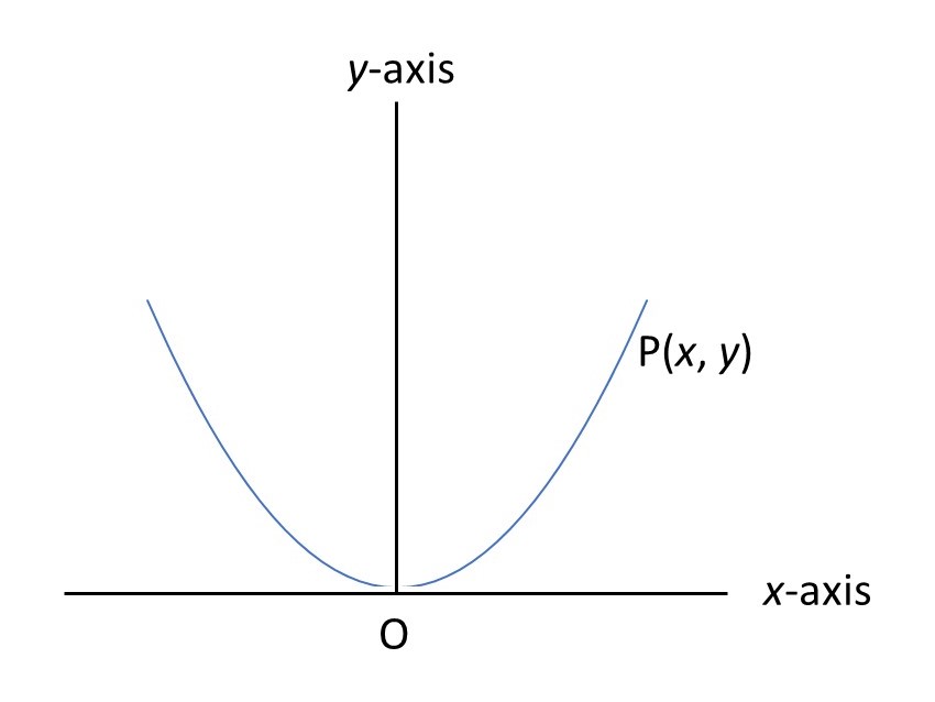
In the picture above, the axis of the symmetrical curve (coloured blue) defines the y-axis of a Cartesian coordinate system whose origin is at the minimum of the curve. The x-axis makes a right-handed set. P is a point on the curve with coordinates (x, y); the type of curve defines how y depends on x. The three-dimensional concave surface is formed by rotation about the y-axis to form a dish-shaped object.

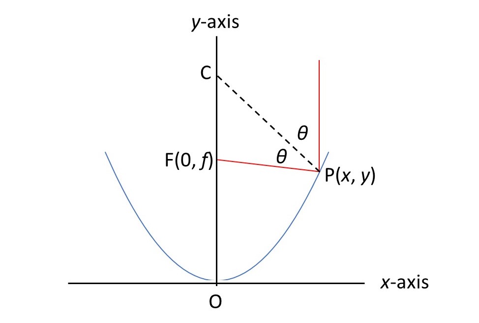
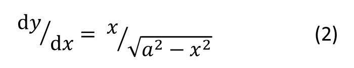
In the picture above, the axis of the dish points in the direction of the source. A ray parallel to this direction that meets the dish at P is reflected and meets the axis at F; the coordinates of F are defined to be (0, f), since it lies on the y-axis. The dotted black line is perpendicular to the tangent to the curve at P. Then, since the angle of incidence is equal to the angle of reflection, PC makes equal angles of θ with the incident and reflected rays. (You may have noticed that C is the centre of curvature of the curve at P so CP is the radius of curvature – if you haven’t, it doesn’t matter). In appendix 1, I show, for any curve that is symmetric about the y-axis, that

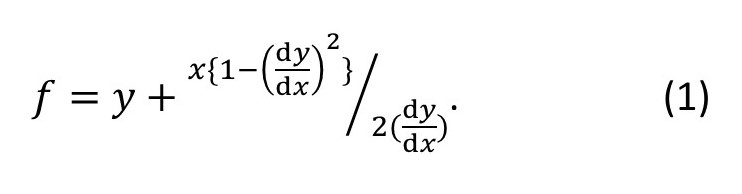
Here dy/dx is the slope of the curve at any given point that is equal to the slope of the tangent to the curve at that point, as explained in post 17.4.

Now let’s suppose that the blue curve, in the pictures above, is the arc of a circle of radius a, as shown in the picture above. In appendix 2, I shown that

and, in appendix 3, that

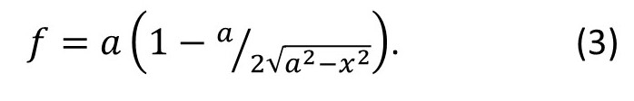
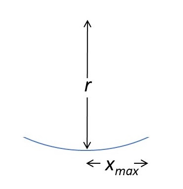
We can see that f depends upon the value of x, that is on the position of P. But let’s suppose that a is much greater than the maximum value, x_max, possible for x, as shown in the picture above. Then equation 3 approximates to

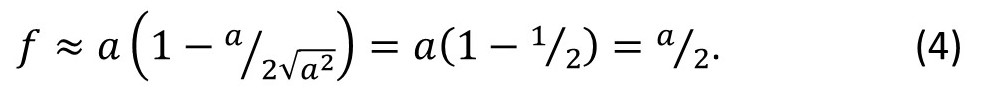
Now all parallel rays cross the y-axis at a distance of a/2 from the origin. Of course, equation 3 is an approximation. As the size of the mirror increases, this approximation fails. The failure of the approximation that causes F to depart from a point, for a curved mirror or for a lens, is called spherical aberration.

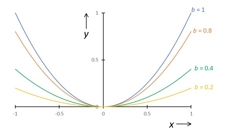
Now let’s suppose that the blue curve is a parabola and not an arc of a circle. The parabola is defined by the equation

y = bx²

as shown in the picture above; this picture shows how the value of b influences the appearance of a parabola. When this curve is rotated about the y-axis, it generates a three-dimensional shape called a paraboloid. Then

dy/dx = 2bx.

If we substitute the expressions for y and for dy/dx for a parabola into equation 1, we get

Since b is a constant, for a given parabola, equation 5 shows that f is now at a constant distance from the origin. This means that a parabolic reflector has a fixed focal point and has no spherical aberration.

In our examples of radio-telescopes, Radar receivers, mobile phone masts and satellite dishes, there is a detector at F. Rays from a distant object, that are effectively at an infinite distance, are then focussed at F by a parabolic reflector. In a searchlight, there is a source of light at F and a parabolic mirror produces a parallel beam of light.

Related posts

22.4 Reflection
22.1 Refraction at curved surfaces

Follow-up posts

22.7 The caustic curve

Appendix 1

The purpose of this appendix is to derive equation 1.

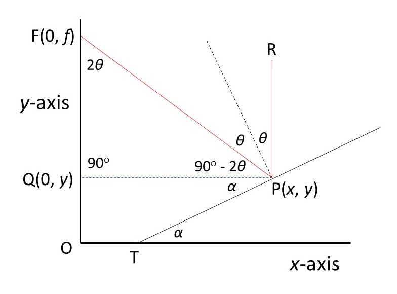
In the picture above, P is a point on a concave mirror that reflects the ray RP along the path PF, where F is defined in the main text. TP is the tangent to the curve at P and the dotted black line is perpendicular to TP. The blue dotted line PQ is parallel to the x-axis.

The angle of reflection is equal to the angle of incidence, θ. Since RP is perpendicular to PQ, the angle FPQ is equal to 90^o – 2θ. Since the dotted black line is perpendicular to TP,

α + (90^o – 2θ) + θ = 90^o   or   α = θ.

Since QP is parallel to the x-axis, TP makes an angle of α = θ with the x-axis (if it didn’t QP would eventually meet the x-axis). Then the slope of the curve at P is given by (see post 17.4)

tanθ = dy/dx = tanα.                    (A1)

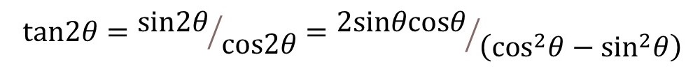
Since the sum of the angles in triangle PQF is 180^o, the angle PFQ is equal to 2θ. From the definition of the tangent of an angle

tan2θ = x/(f – y)

so that

f – y = x/ = x(1 – tan²θ)/(2tanθ).                    (A2)

The final step uses the relationship

derived in appendix 4. Substituting the expression for tanθ from equation A1 into A2 gives equation 1.

Appendix 2

The purpose of this appendix is to derive equations 2.

If a Cartesian coordinate system has its origin at the centre of a circle of radius a, and (X, Y) is a point on the circumference of this circle, then

X² + Y² = a²                    (B1)

as shown in post 21.3. In this coordinate system X = x and Y = y – a, where x and y are defined in the coordinate system of the main text. Substituting these relationships into equation B1 gives

x² +(y – a)² = a²

that can be written (see appendix 4 of post 17.4) as

x² + y² – 2ya + a² = a²

which simplifies to

x² + y² – 2ya = 0.                    (B2)

Solving equation B2, which is a quadratic equation, for y gives

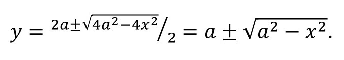
For the blue curves that form our reflecting surfaces, y must be less than a, so we choose the solution

y = a – (a² – x²)^1/2.                    (B3)

Here I have used the subscript ½ as an alternative to the square root sign, as described in post 18.2. To obtain equation 2, we need to differentiate equation B3 as described in post 17.4.

First, I define   u = a² – x²   so that   y = a – u^1/2   and   du/dx = -2x. Then   dy/du = -(1/2)u^-1/2.

Since   dy/dx = (dy/du).(du/dx)   (see post 17.13) we can write

dy/dx = x(a² – x²)^-1/2

which is another way of writing equation 2.

Appendix 3

The purpose of this appendix is to derive equation 3.

According to equation B2

y = a – (a² – x²)^1/2 = a – w                    (C1)

where w is defined by equation C1 as

w = (a² – x²)^1/2 = a – y                    (C2).

According to equation 2

dy/dx = x(a² – x²)^-1/2 = x/(a² – x²)^1/2 = x/w.                    (C3)

The final step uses the definition for w from equation C2.

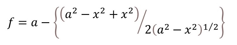
According to equations 1 and C2

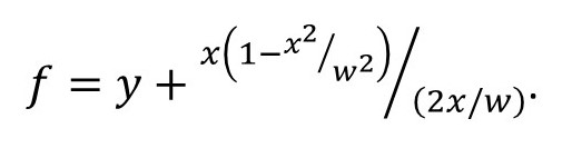
Simplifying this result gives

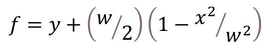
or

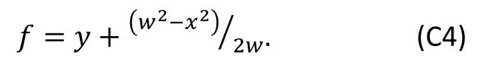
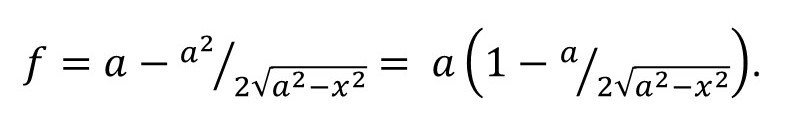
From equations C1 and C4

Now substituting the definition of w, from equation C2, into this result gives

or

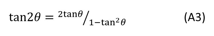
Appendix 4

The purpose of this appendix is to derive equation A3.

From the definition of the tangent of an angle

where the final step uses expressions for the cosine of the sum of angles and the sine of the sum of angles. Dividing the top and bottom of the right-hand side by cos²θ gives

From the definition of the tangent of an angle

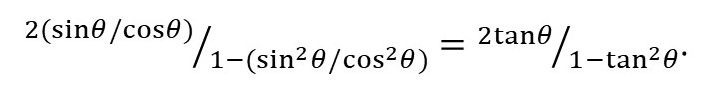
Therefore

.
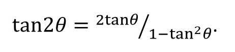