Before you read this, I suggest you read posts 17.15, 20.34 and 20.35.

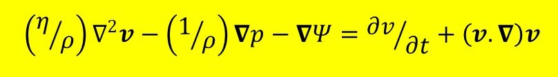
The equation highlighted in yellow, above, is the Navier-Stokes equation for incompressible flow of a fluid. A more complicated form of this equation can be used to explain the flow of compressible fluids. For more information on incompressible and compressible flow, see post 20.35. The Navier-Stokes equation differs from Bernoulli’s equation (post 17.15) in that the viscosity (post 17.17) of the fluid need not be negligible. Also, unlike Bernoulli’s equation, the Navier-Stokes equation is not confined to streamline flow but, in principle, can be used to describe turbulence. It is named after the French engineer Claude-Louis Navier (1785-1836), who was a professor at the Ecole-Polytechnique in Paris, and the Anglo-Irish mathematician Sir George G. Stokes (1819-1903). Stokes was Lucasian Professor of Mathematics at the University of Cambridge – a post that has also been held by Isaac Newton (post 16.11), Paul Dirac (post 19.27), Stephen Hawking (post 16.22) and Michael B. Green (a pioneer of string theory in which sub-atomic particles are treated as vibrating strings).

I was asked to write something about the Navier-Stokes equation to help students studying engineering at a UK university. If you don’t want to understand fluid flow at this level, I suggest that you stop reading now!

In the equation above, the operators ∇² and ∇ are defined in post 20.34. A fluid of viscosity η (post 17.17) and density ρ (post 16.44) flows with a velocity v (post 17.4), as a result of a pressure, p, and a potential function Ψ (post 17.15). The potential function is the potential energy for a unit mass of fluid; so, if the potential energy of the fluid is purely gravitational, Ψ = mgh/m = gh, where m is mass, g is the magnitude of the gravitational field, and h is the height of the liquid above some arbitrarily defined zero value (see post 16.21 for more details). The first term on the right-hand side of the equation is the partial derivative (post 19.11) of the modulus (post 17.3) of v with respect to time, t. In this post all the symbols written in bold are vectors; the others are scalars (post 17.3).

I am not going to derive the Navier-Stokes equation. The derivation is complicated and it is more important to understand what the equation represents. In this post, I am going to compare the Navier-Stokes equation with Bernoulli’s equation; this is the reason for giving the Navier-Stokes equation for incompressible flow at the beginning of this post. In the next post, I will use the Navier-Stokes equation to derive Poiseuille’s equation (post 17.42). But, the Navier-Stokes equation is usually solved numerically, in a technique called computational fluid dynamics (CFD), to predict how fluids will flow. Post 19.17 gives an example of how computer modelling can be used to simulate physical systems. However, the approach in the post differs from that used in CFD, where numerical methods are used to solve a differential equation (post 19.10).

Now we are going to consider laminar flow along the z-direction of an orthogonal Cartesian coordinate system (post 16.50). I will use the unit vectors i, j and k to define the x, y and z axes, respectively, of this system (post 17.3). Since the flow is in the z-axis direction, we can write

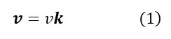
where v is the modulus of v. Then

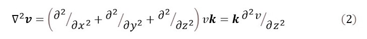
since v has no components in the x and y-directions. Now

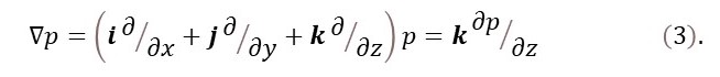
The final step arises because flow is confined to the z-direction, so p cannot change in the x and y-directions. Similarly, since flow occurs only in the z-direction, Ψ cannot change in the x and y-directions, with the result that

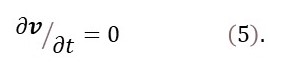
If the fluid flows in streamlines, as described in post 17.15, it cannot accelerate, so that

Now

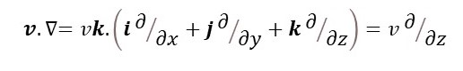
where the first step comes from equation 1 and the next step arises because k.i = k.j = 0 and k.k = 1 (post 17.3). Then

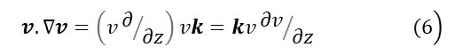
since k is a constant.

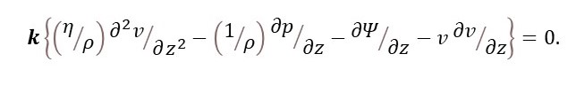
Substituting equations 2, 3, 4, 5 and 6 into the Navier-Stokes equation gives

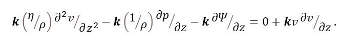
We can write this result as

Now we are going to integrate (post 17.19) this result with respect to z, with the result that

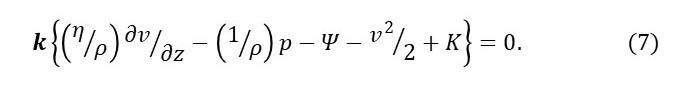
K is the sum of all the constants of integration arising from evaluating four indefinite integrals (post 17.19).

I have written this paragraph in case you can’t see where the v²/2 term has come from. Remember, we integrated equation 6 with respect to z. Then

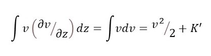
where K’ is a constant of integration. Since k is a vector whose modulus is the number 1 (post 17.3), the only way that the left-hand side of equation 7 can be zero is if

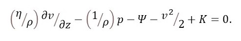
Let’s rewrite this result as

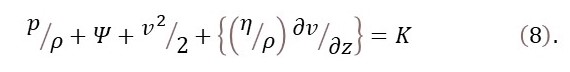
Equation 8 is the same as Bernoulli’s equation except for the term in {curly brackets}. This final term allows for energy dissipated by the flow of the viscous fluid (post 17.17). When the viscosity is negligible, η= 0, so that the last term in equation 8 is zero and the result is identical to Bernoulli’s equation in post 17.15.

In conclusion, if we apply the Navier-Stokes equation to laminar incompressible flow, we get a result that has the same form as Bernoulli’s equation but includes a term that allows for energy dissipated by viscous flow. When the viscosity is negligible, the Navier-Stokes equation and Bernoulli’s equation are identical for laminar incompressible flow.

Related posts

17.15 Fluid flow
20.35 Incompressible and compressible fluid flow

Follow-up posts

https://thinking-about-science.com/2020/10/11/20-37-poiseuilles-equation/