Before you read this, I suggest you read post 22.12 and appendix 3 of post 22.20.
When you read the title, this may seem like a very obscure topic. But it isn’t because we need to understand the Fourier transform of a lattice to understand x-ray diffraction by a crystal. And we need to understand x-ray diffraction by a crystal to understand x-ray crystallography – one of the most important techniques for determining the structures of molecules.
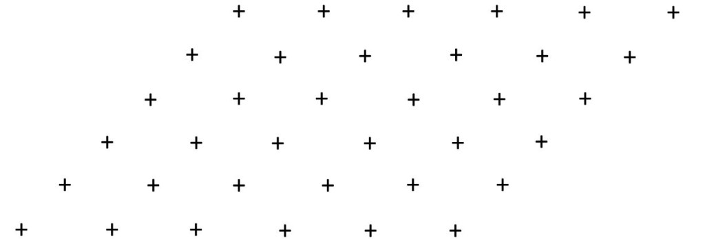
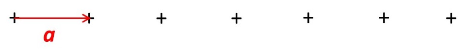
In post 22.21 we saw that a lattice was a regular arrangement of points in space – like the two-dimensional example in the picture above, where the centre of each cross marks the position of a point. The picture below shows a one-dimensional example where there is a vector a separating each atom from the next. In this post we shall investigate the Fourier transform of this one-dimensional lattice; in a later post, we will use this result to find the Fourier transform of a three-dimensional lattice.
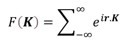
We can represent each point as a Kronecker delta function, δ(r), whose value is 1 at each of the lattice points and zero elsewhere. Then the Fourier transform of the lattice is no longer a continuous function but is the sum of the contributions of each point
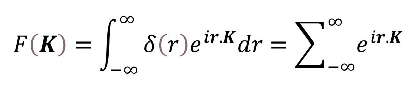
If this seems difficult to understand read appendix 1. Here i is the square root of -1 (post 18.16) and K is the vector that defines the space in which we plot the Fourier transform (see appendix 1 of post 19.20); r.K denotes the dot product of the vectors K and r where r is a vector in the direction of the lattice points. The number e has a value of about 2.718.
At this point you may be concerned that I am using the Kronecker delta function instead of the more rigorously defined Dirac delta function; if you are – see appendix 2. The reason that I chose to use the Kronecker delta function here is that I think it is easier to understand.
Now we are going to suppose that there are n + 1 points in our one-dimensional lattice and place our origin at the first point. Then
F(K) = 1 + eia.K + e2ia.K + e3ia.K + e4ia.K + ………………………..+ enia.K.
In this series, each term is generated from the previous term by multiplying it by the same thing (in this case eia.K). A series like this is called a geometric progression; in appendix 3 we see how to add all the terms in a geometric progression – applying the result here gives
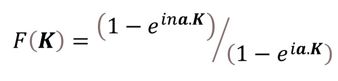
This result can be written as
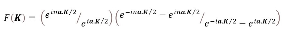
If you find this difficult to follow, it might help to read about powers of numbers in post 18.2. Finally
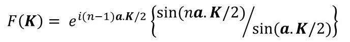
where this final step involves expressing the sine of an angle as the difference between two exponential functions, as described in appendix 2 of post 22.8.
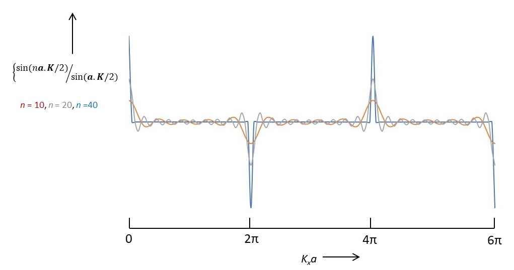
I am now going to show that, as n tends to infinity, the term in {brackets} is non-zero only if
a.K = 2πh (1)
where h is an integer. Here I will use a numerical method; in appendix 4 I shall obtain the same result analytically. In the picture below, I plot the term in brackets for different values of n; you can see that, as n increases, our term increasingly resembles a series of peaks (positive or negative) spaced 2π apart. In this picture Kx is the component of the vector K in the direction of a. This result means that, when n is infinite, F(K) is non-zero only when K satisfies equation 1. The reasons for considering n to be infinity are described in post 22.21.
The pictures below shows that equation 1 represents a series of planes, perpendicular to the line of lattice points, spaced a distance 2π/a apart. But you will notice that the origin is now the origin that I have chosen as the origin for the K vectors – it is not the origin that we used to describe the position of the lattice points. We call this origin, O’, the origin of K–space. K-space is an important concept for understanding diffraction and I shall write more it in the next post.
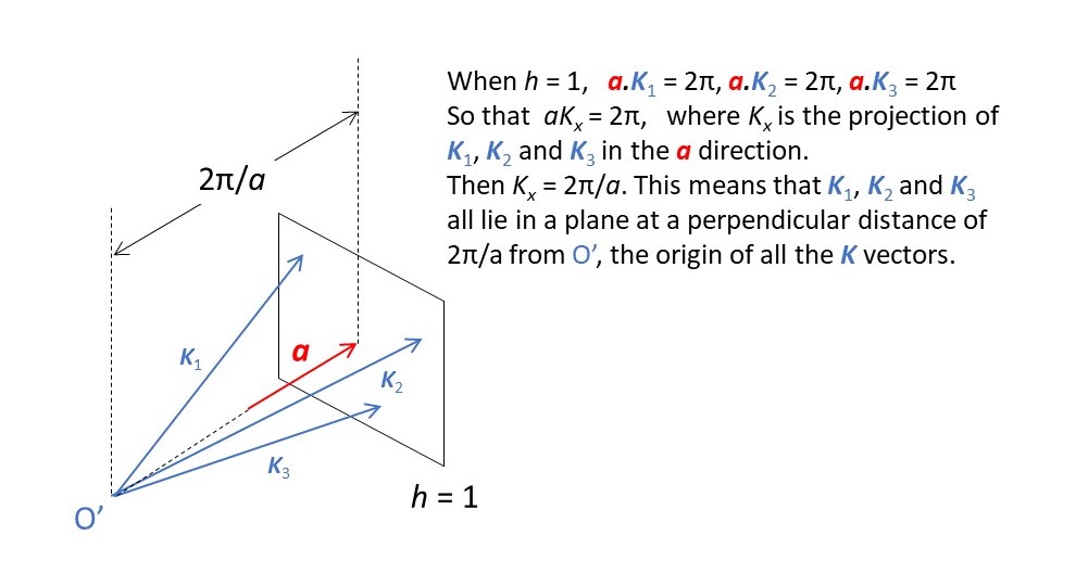
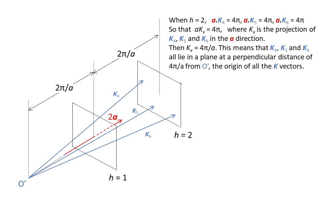
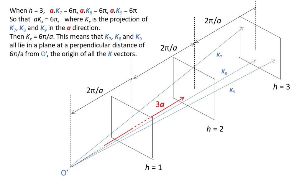
When you’re looking at the above pictures, don’t forget that h can equal 0 (a plane perpendicular to a that includes O’ or be negative (planes on the other side of O’).
We conclude that F(K), the Fourier transform of the one-dimensional lattice, is non-zero only on a set of planes spaced 2π/a apart in K-space.
Related posts
22.21 An ideal crystal
22.12 Diffraction, Fourier transforms and image formation
Follow-up posts
22.23 K-space
22.24 Reciprocal lattice
23.01 Observing x-ray diffraction by a crystal
23.03 X-ray diffraction by a crystal
23.08 Frequency analysis
Appendix 1
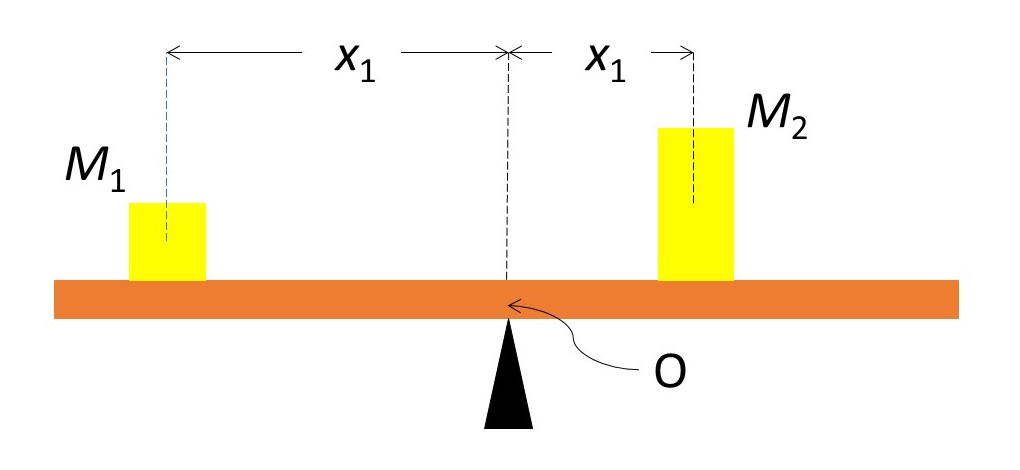
Think of a horizontal beam that is balancing about the point O in the picture above. The beam supports two masses, M1, a distance x1 from O and M2, a distance x2 from O. If the mass of the beam is negligible and the system is in equilibrium, we can sum the torques to obtain
M1x1g + M2x2g = 0 A1
where g is the modulus of the gravitational field. Note that, taking O to be the origin, x1 has a negative value.
We say that the beam is balanced about O because O is the centre of gravity of the system. The position of the centre of gravity is defined by equation A1 that we could generalise, for a system of discrete masses by the sum over all n masses in the system written as
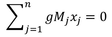
The summation defines the position of the centre of mass of the system to be at O. If the mass distribution along the beam were not centred at discrete points but instead was a continuous function of x, we would write this result as the definite integral
where the limits of integration are over the whole system, as described in post 17.23.
The use of a summation for discrete points and an integral for a continuous distribution is identical to their use in the main post.
Appendix 2
I am now going to show that
using the Dirac delta function, instead of the Kronecker delta function. Our lattice of n + 1 points can be described by
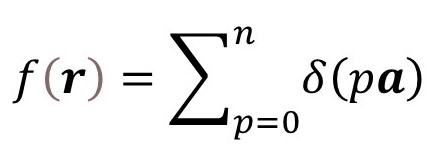
and its Fourier transform is
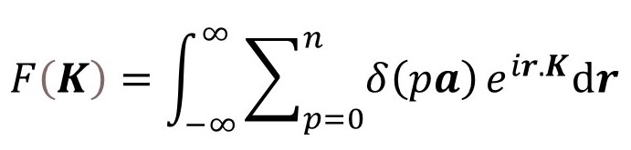
Now remember that the summation is over discrete points. So let’s think about each individual point – for example when p = 3. For this point
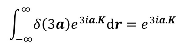
from the definition of the Dirac delta function. When we add the results for each discrete point together, we get
F(K) = 1 + eia.K + e2ia.K + e3ia.K + e4ia.K + ………………………..+ enia.K.
which is the same result that we got using the Kronecker delta function.
Appendix 3
We can represent a geometric progression by
p + pr +pr2 + pr3 + pr4 + ……..
Then the sum of the first n terms is given by
Sn = p + pr +pr2 + pr3 + pr4 +…+ prn-1
so that multiplying by r gives
rSn = pr +pr2 + pr3 + pr4 + pr5 +…+ prn
and subtracting rSn from Sn gives
(1 – r)Sn = p – prn
or
Sn = p(1 – rn)/(1 – r).
Appendix 4
Our infinite one-dimensional lattice can be described by the function f(r), as in appendix 2. Since this lattice is infinite
f(r) = f(r + a)
Calculating the Fourier transform of both sides of this equation gives
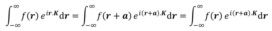
But this result is true only if
eir.K = ei(r + a).K or (dividing both sides by eir.K) 1 = eia.K
Applying Euler’s relation
cos(a.K) + isin(a.K) = 1
From the properties of the sine and cosine of an angle (see post 16.50), this can only be true if
a.K = 360o × h
Expressing the angle in radians gives
a.K = 2πh
