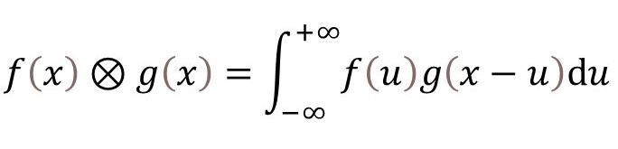
The convolution of two functions of x, f(x) and g(x), is defined by the definite integral

Convolution is defined mathematically but it is possible to understand what it means in pictures. So, if you don’t like mathematics, ignore the next paragraph and the appendices.

The definition of convolution can be extended into two, or more dimensions, to give, for the two-dimensional example

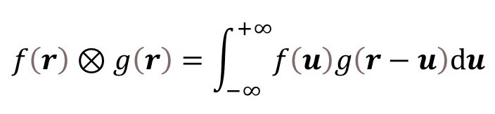
where r is a two-dimensional vector whose components are x and y and u is a two-dimensional vector with components u₁ and u₂ in the x and y-directions, respectively; the limits of integration are over both u₁ and u₂. I will use only one-dimensional convolution in this post but the results apply to two or more dimensions.

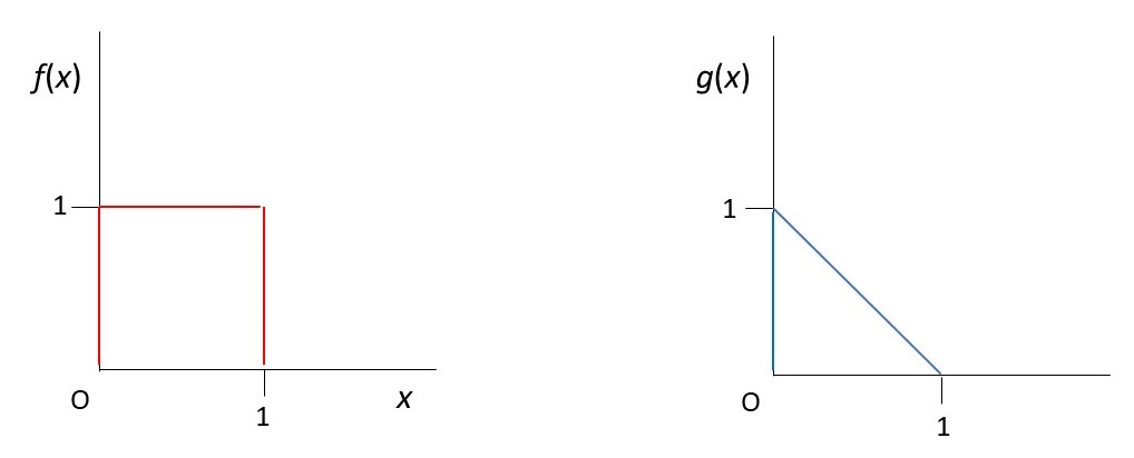
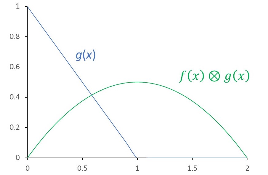
What does the convolution of two functions look like? The picture above shows two functions f(x) and g(x). The picture below shows the convolution of the two functions.

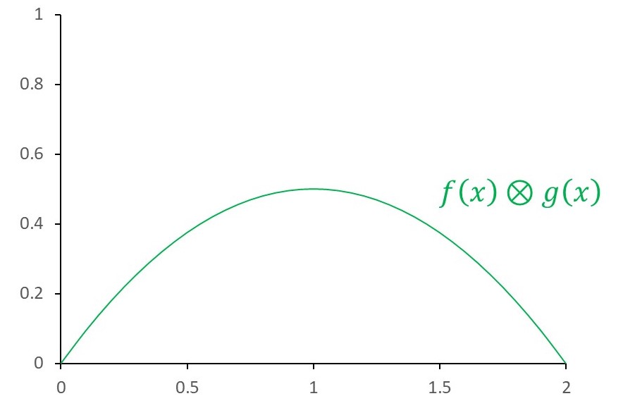
If you want to see how this result was calculated, see appendix 1. The picture below compares g(x) before and after convolution with f(x).

Before convolution g(x) had a very sharp peak – now the peak is blurred and moved along the x-axis.

The effect is like moving a camera when you’re taking a picture of something. We can think of the blurred picture as the convolution of an image the object, g(x), with the convolution of a function, f(x), that describes the movement of the camera. Correction of blurred photographs involves recovering g(x) by reversing the operation of convolution usually by trying different forms for f(x) until a sharp image is obtained – this process is called deblurring or deconvolution.

If we reverse the order of convolution, the result is the same, so that

When the order of a mathematical operation is unchanged by the order in which it is applied, we say that it is commutative. Multiplication of ordinary numbers (scalars) is commutative because, for example, 3.47 × 18.6 = 18.6 × 3.47. In appendix 2, I give a mathematical proof that the convolution of two functions is always commutative.

Now we are going to see what happens when one of our functions represents a point in space (marked by a diagonal cross). In the picture below, I convolute a smiley function with a single point. The result is to set down the smiley function with the point as its origin, as shown in the picture below. This result is proved in appendix 3.

Below we convolute a smiley with a line of three points – we set down the smiley with each point as an origin.

And below is a two-dimensional example – convolution of a smiley with three points that are not in a straight line.

So we have seen two applications of convolution. One: to describe blurring of an image. Two: to build repetitive images of an object.

A third application is more mathematical: convolution can be used to simplify the calculation of a Fourier transform. Fourier transforms are explained in post 22.12 but I will give a simple explanation here. Like convolution, Fourier transformation, involves evaluating a definite integral between plus and minus infinity. The Fourier transform is used to find the sine and/or cosine waves that can be added together to form some function h(x). So, it resembles a Fourier series but, unlike a Fourier series, the function is not periodic. We can represent the process of Fourier transformation by the letter T so that T[h(x)] is the Fourier transform of h. The convolution theorem states that

and is proved in appendix 4. If h(x) can be expresses as the convolution of f(x) and g(x), the convolution theorem may help us to calculate h(x) more simply. So a third application of convolution is to simplify the calculation of some Fourier transforms.

Related posts

22.12 Diffraction, Fourier transforms and image formation

Appendix 1

Convolution of the functions f(x) and g(x).

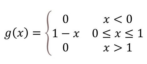
The equations of f(x) (the red curve in the graph) and g(x) (the blue curve) are given below.

Then

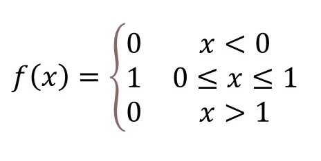
because, outside these limits, f(u) = 0. Within these limits, f(u) = 1. Then

Evaluating this definite integral gives

Appendix 2

Convolution is commutative

By definition

Let’s define v = x – u so that u = x – v and du/dv = -1. Now the integral becomes

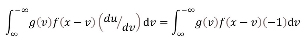
Why have I changed the limits of integration? Because, for a given value of x, v gets smaller as u gets bigger. We can write the second integral as

So convolution is commutative.

Appendix 3

Convolution of a function with a point in space.

We will think about convolution of a one-dimensional function, s(x), with a single point that, for simplicity, we can define to have x = 0, that is, it defines an origin. Now a delta function is defined by δ(x) = 0 when x ≠ 0.

The simplest form of the delta function is called the Kronecker delta function, after the German mathematician Leopold Kronecker (1823-1891). It is defined as

Then, from the definition of convolution

But this integral is non-zero only when δ(u) is non-zero, that is at the point u = 0. At that point, our integral becomes

since δ(u) = 1 when it is non-zero. Here Δu is the width of the point. But, by definition, a point in space has no width so Δu = 0 with the result that δ(x)⨂s(x) is zero.

It seems that something has gone wrong! Why? It is really a problem with the Kronecker delta function. This problem disappears when we use the definition of the delta function attributed to the British physicist Paul Dirac.

The Dirac delta function is defined by the area under a curve, so that

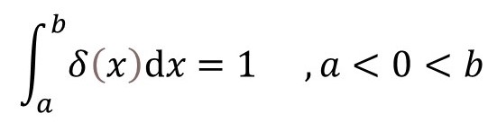
otherwise the value of the integral is zero. Now our convolution becomes

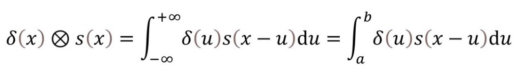
because the Dirac delta function would be zero outside these limits. When u = 0, s(x – u) = s(x) and its value is independent of u. So our convolution integral becomes

from the definition of the Dirac delta function. Remember that the origin we are using is the original point whose position defined the position of the delta function.

So, the effect of convolution was to put the origin of s(x) at this point.

Appendix 4

The convolution theorem

From the definitions of convolution and the Fourier transform

where K defines the K-space of the Fourier transform (see post 22.12).

Now I’m going to define v = x – u so that du/dv = -1. Then the result above becomes

Note that we have changed the limits of integration of the inner integral for the same reason as in appendix 2. Then this result can be written as

The final result is T(f) × T(g).