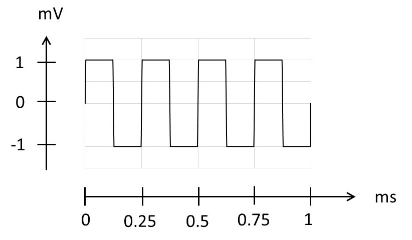
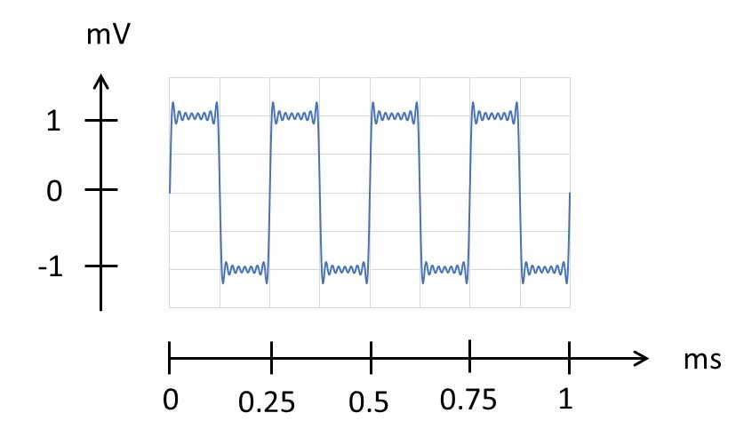
Let’s think about a wave, that we can represent by a wave function ψ(t) where t represents time, that has a time-period is T. An example is the time-dependent electrical potential, shown above (see also post 18.14) that has T = 0.25 ms.

The Fourier transform of this one-dimensional function is defined by

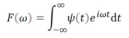
This is directly analogous to the calculation of the Fourier transform of a one-dimensional lattice in post 22.22. In post 22.22, the Fourier transform was plotted as a function of a variable K. Here, I am considering it as a function of a variable, ω, to emphasise that the function being transformed here varies in time and not (as in post 22.22) in space. If you are comparing this post with post 22.22, you may wonder why I used a vector equation there but not here. It is because, in post 22.22, K represented a scattering vector that was not confined to the direction of the function whose transform was being calculated. Here ω is simply a variable that I’ve introduced to plot a one-dimensional Fourier transform – although we shall soon see that it has a physical significance.

Using the same reasoning as in post 22.22, we find that, F(ω) is non-zero only when ω_n = 2πn/T, where n is an integer, so that ω_n represents an angular frequency. If this isn’t clear, put n = 1 and then see the definition of ω in post 17.12.

Using Euler’s relation, we can write F(ω) as the sum of real and imaginary parts

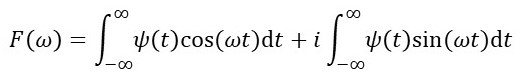
where i is the square root of -1.

In post 18.14, we saw that any periodic function could be represented by a sum of sine and cosine waves, called its Fourier series, so that

It turns out that the coefficients a_n and b_n are given by the real and imaginary parts of F(ω), respectively. So the Fourier transform tells us the contributions to ψ(t) of sine and cosine waves of different frequencies – it performs a frequency analysis. In practice, we cannot add an infinite number of discrete terms so that we replace infinity by N where N is very large. In post 18.14, we represented a square wave reasonably well using N = 15, as shown in the picture below.

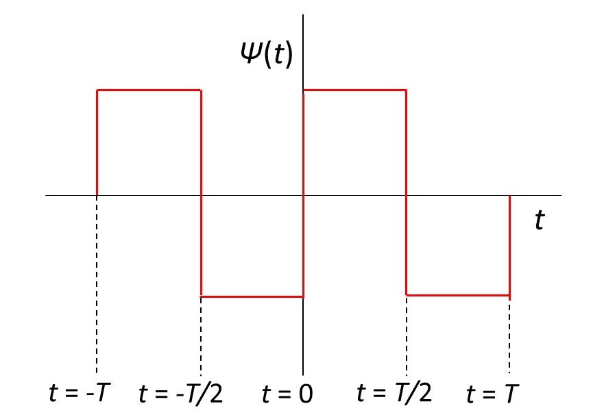
The picture below shows two cycles of a square wave, ψ(t), (see the picture above) with a time period T. By defining the origin at the point shown in the picture, ψ(t), is defined as an odd function (like sine) that is ψ(t) = – ψ(-t). By contrast, a function like cosine is an even function because cos(t) = cos (-t) (see post 16.50).

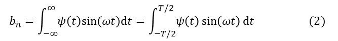
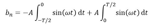
So, we can represent ψ(t) by adding a series of sine waves, as shown in the first picture of this post. The coefficients that we use to form ψ(t) from these sine waves is given by the imaginary part of F(ω), that is

The final step follows because the wave simply repeats itself.

We can represent a square wave, of amplitude A, by

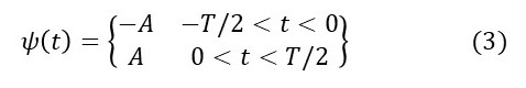
Substituting equation 3 into for equation 2 gives

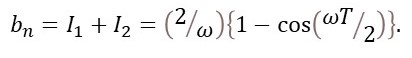
Evaluating this definite integral gives

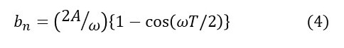
(see the appendix). Using the relationship between the time period and angular frequency, equation 4 becomes

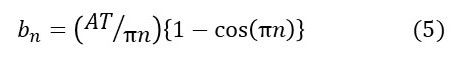
The table below shows values of b_n and ω_n for different values of n.

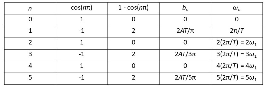
Substituting these values for b_n and ω_n into into equation 1 gives

I used equation 6 (in post 18.14), putting A = 0.5 (to scale the result to give a peak of 1 mV) and T = 0.25 ms, to construct a square wave. Now we know how it was derived. Note that n = 1 defines the fundamental frequency and n = 3, 5, 7… are its harmonics. If we hadn’t recognised that our square wave was an odd function, we could have used the real part of F(ω) to calculate a_n and we would have then found that it is always equal to zero.

What happens when we add a constant to the sum of sine and/or cosine waves in a Fourier series? The result is that we see the oscillations about a different baseline, as shown in the picture above. This picture is the same as the second picture in this post except that a constant voltage of 1 mV has been added. Let’s think about the result of our time-dependent electrical potential. It can produce a time-dependent current. A current that oscillates about zero amps is called an alternating current, usually written as AC. A current that is constant is called a direct current, usually written as DC. Adding a constant to the sine waves that represent our time-dependent voltage represents the effect of adding a voltage that produces a direct current and so is sometimes called a DC term.

In the next post we will look at frequency analysis of a signal that we can’t represent by a simple function like ψ(t).

Related posts

18.14 Wave shapes

Appendix 1

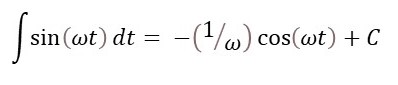
where C is a constant of integration. You can confirm this result by calculating the derivative of the right-hand side. Now let’s define the definite integrals I₁ and I₂ by

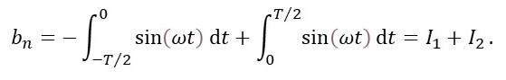
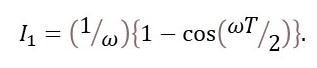
Then

Noting that the cosine of zero is 1 and that the cosine of a negative angle is equal to the cosine of a positive angle (post 16.50), this becomes

And

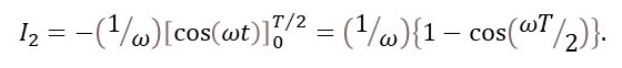
Then