Before you read this, I suggest you read posts 22.22 and 22.23.

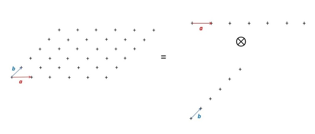
In post 22.22, we saw that a one-dimensional lattice was a line of points, each separated by the vector a. The picture above shows how a two-dimensional lattice can be generated by convolution of two one-dimensional lattices. A three-dimensional lattice can be generated by convolution with a third one-dimensional lattice whose points are each separated by a vector c. The vector c points out of the plane of the picture but not necessarily perpendicular to it. The vectors a, b and c form a right-handed coordinate system that is not necessarily orthogonal. These vectors are the unit cell vectors of an ideal crystal.

The concept of a reciprocal lattice arises when we calculate the Fourier transform of a two or three-dimensional lattice.

Since these lattices can be considered as the convolution of two or three one-dimensional lattices, their Fourier transforms can be multiplying the Fourier transforms of one-dimensional lattices – as explained in post 22.20.

The Fourier transform of our first one-dimensional lattice of points separated by a, is non-zero only on a set of planes, perpendicular to a, spaced a distance 2π/a apart in K-space (see post 22.22). The Fourier transform of our second one-dimensional lattice of points separated by b, is non-zero only on a set of planes, perpendicular to b, spaced a distance 2π/b apart in K-space. In the two dimensions of the picture below, these planes appear as red and blue lines.

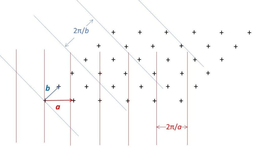
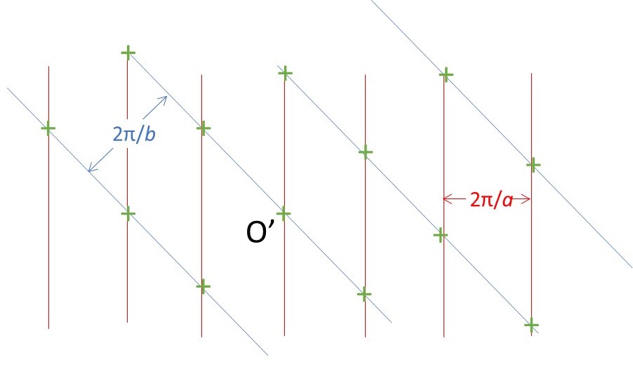
When we multiply these Fourier transforms, the result is non-zero only on the lines generated by the intersection of the planes. In the two dimensions of the picture above, these planes appear as lines that intersect at the points marked by green crosses. This set of points is called the reciprocal lattice. The picture below shows a two-dimensional reciprocal lattice but we are usually interested in the three-dimensional case when the two sets of planes are multiplied by a third set, perpendicular to c, spaced 2π/c apart in K-space. Then the result is non-zero only at a set of points where the planes intersect in three-dimensional K-space.

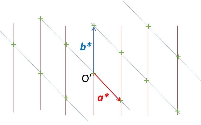
We define the reciprocal lattice vectors, a*, b* and c*, in reciprocal space in the same way that we define the unit cell vectors, a, b and c, in real space – as shown (in two dimensions) in the picture above. The positions of the points in a two-dimensional reciprocal lattice can be indexed by the values of two integers h and k, as shown in the picture below. The origin of K-space, O’, defines the position of the point indexed by h = 0 and k = 0. For a three-dimensional reciprocal lattice, we need a third integer, l. These integers, h, k and l, are called Miller indices and are named after the Welsh mineralogist William Miller (1801-1880).

Then the position of a reciprocal lattice point with Miller indices h, k and l is given (in K-space) by

K = ha* + kb* + lc*.

Note that a* lies in a plane that is perpendicular to a and that the reciprocal lattice points, along the a direction, are formed by parallel planes spaced a distance 2π/a apart. So, if we form the dot product of the vectors a* and a, the result is

a*.a = 2π.

Similarly

b*.b = 2π    and   c*.c = 2π.

But, for example, a* is perpendicular to b and to c (you can see this, in two-dimensions from the pictures above). When we think also about b* and c* we can write all the dot products as

a*.a = 2π      a*.b = a*.c = 0

b*.b = 2π      b*.a = b*.c = 0

c*.c = 2π      c*.a = c*.b = 0

This set of equations can be used to calculate the reciprocal lattice vectors from the unit cell vectors. The equations are called the Laue equations after the German physicist Max von Laue (1879-1960).

If you read about the reciprocal lattice in most textbooks on crystallography you may be confused by the appearance or disappearance of a factor of 2π from my equations. This is because most of these books use reciprocal space, instead of K-space, that is defined by a vector S where S = (1/2π)K.

Assigning Miller indices to reciprocal lattice points is an essential step in determining the structure of a molecule by x-ray crystallography. And understanding the concept of the reciprocal lattice is important for understanding x-ray diffraction by a crystal.

Related posts

22.12 Diffraction, Fourier transforms and image formation
22.20 Convolution
22.21 An ideal crystal
22.22 Fourier transform of a one-dimensional lattice
22.23 K-space

Follow-up posts

23.01 Observing x-ray diffraction by a crystal
23.03 X-ray diffraction by a crystal