I mentioned the idea of K-space in post 22.22 and introduced the vector K in post 19.20; in post 22.12 I described the Fourier transform as a function of K. The purpose of this post is to bring all these ideas together.

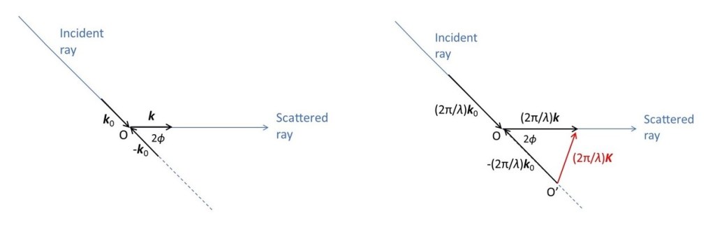
In the left-hand picture above, a ray is scattered by a particle at O. Let’s think about the ray scattered, through an angle 2ϕ by the particle. Following post 19.20, I will define the incident direction by a unit vector k_o and the scattered direction by the unit vector k. The change in direction of the ray is given by (k – k_o). I am now going to define the vector K by

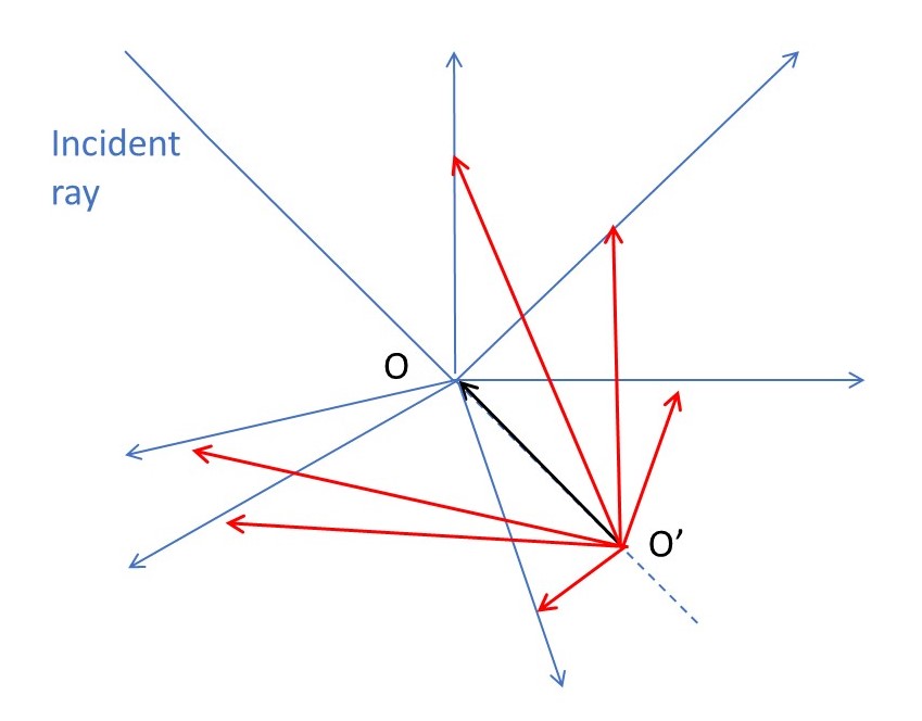
K = (2π/λ)(k – k₀)                    (1)

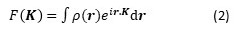
as shown in the right-hand picture above. Here λ represents the wavelength of the ray, for the reasons given in post 22.14. The picture below shows that, for all scattering directions, the origin of the K vectors is at O’ that lies in the direction of k a distance 2π/λ from O, when the direction of the incident ray doesn’t change. Of course, scattered rays and, therefore, K vectors are not confined to the plane of the picture, which is a two-dimensional representation of something that happens in three dimensions. In post 19.20, we saw that the modulus of K is given by

K = (4π/λ)sin(ϕ/2).

The vectors K define a space, called K-space, whose origin is at O’. If we multiply our definition of K, in equation 1, by 2π the resulting vector defines what is sometimes called reciprocal space.

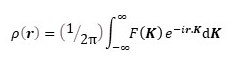
In posts 22.12 and 22.14, we saw that the rays scattered by an object (its diffraction pattern) could be represented, in amplitude and phase by the Fourier transform, F, of the density of scattering matter, ρ, in the object. F is a function of K and is defined by

                   

where the limits of integration are over the volume of the scattering object. Here r is a vector defining positions in the scattering object so that ρ is a function of r. We define the origin of the r vectors to be at O. Then the vectors r are in real space, whose origin is at O.

Let’s explore the relationship between K-space and real space in more detail.

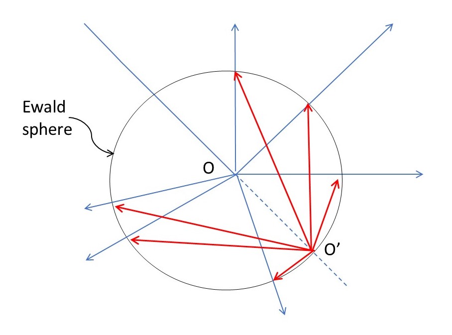
From the definition of K, in equation 1, all possible K vectors define a sphere of radius 2π/λ, whose centre is at O, the origin of real space, as shown in the picture above (where the K vectors are shown in red). The picture shows a circular section of this sphere because it is a two-dimensional representation of what happens. This is because the points of the red arrows are all a distance of (2π/λ) from O. Equation 2 implies that K-space has an infinite extent but the picture shows that, for a fixed position of the scattering object, we can only explore the region of K-space that lies on the surface of this sphere – called the Ewald sphere after the German physicist Paul Ewald (1888-1985).

We can explore more of K-space by rotating the object in real space – leading to an equal rotation, about a parallel axis, in K-space. Then further regions of K-space pass through the Ewald sphere – providing more information about the object. But we can only explore regions of K-space for which K < 2π/λ which limits the resolution of the information we can obtain with a given wavelength – if we want to obtain higher resolution information, we must extend the region of K-space that we can explore by increasing 2π/λ, that is by decreasing λ. This is the conclusion we reached, by a different route, in post 22.13.

The ideas in the previous two paragraphs are important when we use x-ray diffraction to investigate the positions of atoms in molecules because the radius of curvature of the Ewald sphere is appreciable because the spacing between atoms is comparable to λ. If we use electrons of wavelength 3 pm (see post 22.13), the radius of curvature is much greater so that, for scattering angles not approaching 90^o, the Ewald sphere approximates to a plane section through K-space. Then the diffraction pattern we record is almost a plane section through K-space.

What information does a plane section of K-space provide? Calculating the inverse Fourier transform of equation 2 gives

We can write the dot product r.K as

r.K = xK_x + yK_y + zK_z

where x, y and z are orthogonal Cartesian coordinates in real space and K_x, K_y and K_z, are the components of K in those directions. Now let’s suppose that our plane section is perpendicular to the z-axis, so that

r.K = xK_x + yK_y.

Now

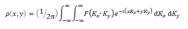
Note that ρ(x,y) is the projection of ρ(r) on the x,y plane. So a section of K-space provides information about a projection in real space.

When we think about diffraction, it is often convenient to think about real space, the space occupied by the scattering object, and K-space, the space occupied by its diffraction pattern.

Related posts

19.20 Diffraction
22.12 Diffraction, Fourier transforms and image formation
22.14 X-ray diffraction
22.21 An ideal crystal
22.22 Fourier transform of a one-dimensional lattice

Follow-up posts

22.24 Reciprocal lattice
23.01 Observing x-ray diffraction by a crystal
23.03 X-ray diffraction by a crystal