In post 24.3 we explored a model of how a population could control itself. This model was based on a differential equation – the most common way to describe how things change with time. This approach was used to describe exponential growth (post 18.15), waves (post 19.12), diffusion (posts 19.15 and 19.16), the behaviour of electrons (posts 19.27 and 19.28), the flow of viscous fluids (posts 20.36 and 20.37), and a simple ecosystem (post 22.17)

Now I am going to use an alternative approach that is mathematically simpler – the application of a recurrence relation. In this approach we consider change to take place in discrete steps or generations. This is similar to the approach I used to introduce exponential growth in post 16.5, although I didn’t explicitly write down the recurrence relation for exponential growth.

As a population grows, there will be factors that tend to control it – for example depletion of food and poisoning by waste products, as described in posts 16.5 and 24.3. Let’s define a generation, consisting of n₀ individuals, to be the initial generation of our population and introduce a variable x₀ that is n₀ divided by the greatest possible number of individuals – before the population is destroyed by the factors that can control it. Successive generations consist of n₁, n₂, n₃, n₄, n₅… individuals and are characterised by x₁, x₂, x₃, x₄, x₅… values that represent the number expressed as a fraction of the maximum possible number. We can calculate the x values for each generation from x₀ by applying the equations below.

x₁ = rx₀(1 – x₀)

x₂ = rx₁(1 – x₁)

x₃ = rx₂(1 – x₂)

x₄ = rx₃(1 – x₃)

x₅ = rx₄(1 – x₄)

and so on, where r is a constant. We can express all the equations, like those above by the single equation

x_i+1 = rx_i(1 – x_i)                    (1)

where i = 0, 1, 3, 4… Equation 1 is an example of a recurrence relation where the value of successive variables are given by the one that went before it. The recurrence relation in equation 1 is called the logistic difference equation.

Where does equation 1 come from? I answer this question in appendix 1.

Since equation 1 and the differential equation I used in post 24.3 are both supposed to model control of population growth, they must be equivalent in some way. I explore this equivalence in appendix 2.

How realistic is it to model the growth of a population in discrete generations? Let’s think about a species of bird that lays eggs only once a year. Now the population really does increase in steps, 1 year apart, and our simple model is a reasonable way to represent growth. But what about a human population that is breeding all the time? Even then we find it convenient to think about generations; for example, the generation born immediately after the second world war (1939 – 1945), to which I belong. We certainly have characteristics in common – in Europe, the first generation to grow up with television and who were teenagers in the 1960s when many social conventions were becoming relaxed. So, even for human populations, thinking in generations, spaced perhaps 10 years apart, can be useful.

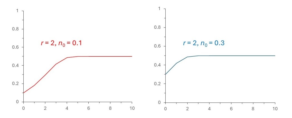
The picture above shows how x_i, for a population varies when r = 2 for two different values of x₀. As we might expect, from post 24.3, x_i settles to a steady number – in this case 0.5.

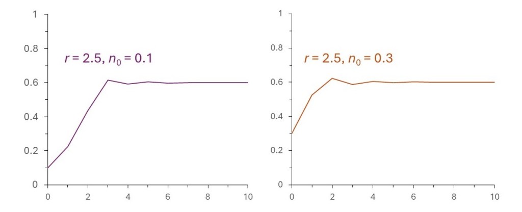
And the picture above, for r = 2.5, shows similar behaviour settling to a constant x_i value of 0.6.

In these examples, the logistic regression equation provides a model for self-controlled growth settling to a constant population..

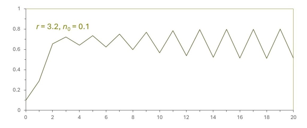
But when r = 3.2 the results are unexpected because x_i oscillates between the two values of 0.5 and 0.8, as shown in the picture above. If you observed this behaviour in a real population you might look for explanations for the increase between generations 13 and 14, for example, or for the decrease between generations 4 and 5. You might even be alarmed that something is going wrong. But you wouldn’t find a simple explanation and there is no cause for alarm – the changes are a result of the value of r for that population. According to appendix 1, it is a result of the rate of increase of the population and the rate at which it decreases. And describing the size of the ith generation by x_i involves the greatest possible number of individuals in the population that depends on factors like the availability of food.

The pictures below show what happens for higher values of r.

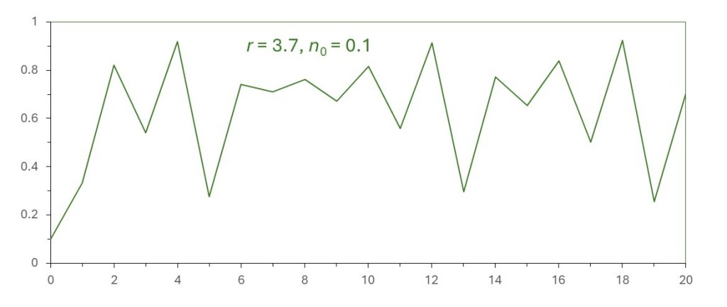
Now equation 1 is showing chaotic behaviour. The result is chaos. What do I mean by “chaos” here? The pattern shown in the picture above is so unpredictable that it appears random. But is isn’t random because it can be predicted if we know that it follows equation 1. This apparently random behaviour is “chaos”.

Populations often show chaotic growth patterns so that a sudden change from one generation to another cannot be explained by a single factor, like the weather or a change in the type of food available or changes in habitat or anything else that we can easily identify.

Related posts

24.3 Limits to growth
22.17 Model for a simple ecosystem

Appendix 1

Derivation of equation 1

We start with a population n₀ and then consider the new population, n₁, some time later. If the population grew uncontrolled we might expect that

n₁ = rn₀,

since, for example, doubling the initial population would be expected to double the population in the next generation; here r is a constant. But, as the population grows, there will be factors that tend to control it – as mentioned above. Initially, these factors may be negligible but, as numbers increase they will become more important. I am going to model the influence of these factors by modifying the equation above to

n₁ = rn₀ – bn₀²

where b is another constant. The second term is negative because it represents a reduction in the population. In the second term I have used the square of the number because the effects that control the population become increasingly more important as the number increases, in the same way that the square of a number increases more rapidly than the number itself. We can represent what happens in each generation by the recurrence relation

n_{i + 1} = rn_i – bn_i²                    (2)

where n_i is the number in the ith generation.

Now let’s introduce another constant defined by k = r/b. Then our recurrence relation becomes

n_{i + 1} = rn_i(1 – n_i/k).

Notice what happens when   n_i = k   so that   n_i/k = 1. Then n_{i + 1} = 0, which means that the population has exceeded its greatest possible size and all the individuals are dead. So when n_i is greater than k, the population will cease to exist and k is the greatest possible number of individuals.

Now dividing each side of the above equation by k gives

(n_{i + 1})/k = (rn_i/k))(1 – n_i/k)   or   x_i+1 = rx_i(1 – x_i).

Appendix 2

Relationship to post 24.3

In post 24.3 we represented the rate of increase, dn/dt, of a population that was subject to self-control by the differential equation

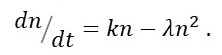
Here n is the number of individuals in the population, t represents time and k and λ are constants.

This differential equation is called the logistic differential equation.

Now let’s think of our population growing in steps from one generation to the next. If n_i is the number of individuals in the ith generation and n_i+1 is the number in the (i + 1)th generation, then the rate of increase is given by

(n_i+1 – n_i)/Δt

which is simply the increase from one generation to the next divided by the time, Δt, between generations.

Comparing this result with our differential equation gives

(n_i+1 – n_i)/Δt = kn_i – λn_i²   or   (n_i+1 – n_i) = Δt(kn_i – λn_i²).

Since there is now a fixed time interval between generations, Δt is a constant and we can write our equation as

n_i+1 = rn_i – bn_i²

where r and b are new constants. This is equation 2 used to derive the logistic difference equation in appendix 1.