Before you read this, I suggest you read post 18.15.

In post 22.17 we saw the effect of predators on the population of a species: the example I used was the natural control of a rabbit population by foxes.

But, in post 16.5, we saw that a population will control itself, without the need for predators, as it starts to consume all the available food and/or it starts to poison itself with waste products. I am going to use the same ideas to understand these self-control mechanisms as I used to look at exponential growth in post 18.15. So, if you are not familiar with the mathematics I use here, most of it is explained there.

We described exponential growth by the differential equation

where n is the number of individuals in the population, t is time, dn/dt is the rate of increase of the population and k is a constant. Solving this differential equation gives us the population at any instant in time. In this example, the population grows increasingly faster.

Now let’s think about how the self-control mechanisms might work. We’ll modify equation 1 to

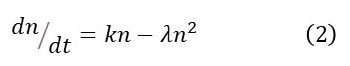
where λ is another constant. The second term on the right-hand side is negative because it represents a decrease, instead of an increase, in the population. I will now explain why I have written n², instead of n, in the second term. When the population is small, self-control will be negligible because there is plenty of food and few waste products. As the population grows there is less food available and waste products start to build up. Then self-control mechanisms become increasingly important. I have attempted to model this effect by using an n² term to model self-control because n² becomes increasingly important as n increases. Equation 2 is sometimes called the logistic differential equation and was developed by the Belgian mathematician Pierre Verhulst (1804-1849).

We can write equation 2 in the form

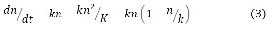
where   K = k/λ.   In appendix 1, I show that solving equation 3 gives

where n₀ is the initial population at some time defined to be t = 0. Appendix 2 shows, from the definition of K, that equation 4 describes exponential growth when   λ = 0   which is what we would expect.

Equation 4 tells us that the population after a time interval, t, has passed depends on

1. n₀ the initial number
2. k the value of the constant of proportionality for growth
3. K the value of k divided by λ, the constant of proportionality for self-control.

The picture above compares the predictions of equation 4 with the corresponding exponential growth model. More details of the calculation are given in appendix 3.

Exponential growth (the blue curve) would accelerate indefinitely. The effect of self-control (the red curve), in the early stages, is to limit the rate of growth and eventually to maintain the population at a stable level.

In general, growth will require resources which become depleted. So there must be limits to the growth of anything.

Related posts

22.17 Model for a simple ecosystem
19.10 Differential equations
18.15 More about exponential growth
18.6 The pendulum: a simple harmonic oscillator
16.6 Exponential decay
16.5 Exponential growth

Follow-up posts

24.4 Logistic difference equation

Appendix 1

Derivation of equation 4.

From equation 3

Integration of this result gives

so that

where C₁ is a constant of integration. In appendix 4, I show that this result can be written as

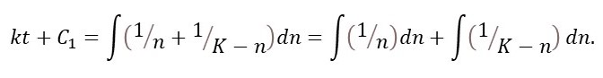
Then

where C₂ is another constant of integration. The calculation of the first integral is explained in post 18.15. In appendix 5, I show how the second integral can be calculated to give

where C₃ is a third constant of integration. Now I define   C = C₂ + C₃ – C₁   so that

n/(K – n) = e^kt + C = Ae^kt                    (5)

where   A = e^C.   If you find this difficult to understand, see post 18.2. Rearranging this result gives

n = (K – n)Ae^kt = KAe^kt – nAe^kt   or   n(1 + Ae^kt) = KAe^kt   or   n = KAe^kt/(1 + Ae^kt)          (6)

A is an arbitrary constant defined by some constants of integration. So I’m now going to use a boundary condition to express it in terms of n₀.

By definition, when t = 0,   n = n₀. Then equation 5 becomes

A = n₀/(K – n₀)                    (7)

since e⁰ = 1. Substituting equation 7 into equation 6 gives

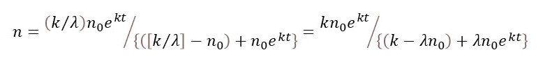
Multiplying the top and the bottom of the right-hand side of this equation by (K – n₀) gives equation 4.

Appendix 2

To show that equation 4 describes exponential growth when λ = 0

From the definition of K, equation 4 can be written

where the final step is obtained by multiplying top and bottom by λ. When λ = 0, this becomes

n = kn₀e^kt/k = n₀e^kt                    (8)

which is the result we obtained from solving the differential equation for exponential growth in post 18.15.

Why bother doing this when the result is exactly what we would expect? The reason is to check that all our ideas and calculations are consistent, in case we’ve made a mistake somewhere.

Appendix 3

Plotting the graph that illustrates equation 4

The blue line was obtained by plotting equation 8 with n₀ = 1000 and k = 0.2.

The red line was obtained by plotting equation 4 with n₀ = 1000 and K = 5000, implying a value of λ = 0.2/5000 = 4 × 10^-5.

These numbers were chosen simply to make it easy to plot a graph comparing the behaviour of these functions.

Appendix 4

To show that

Appendix 5

To show that

Here C₃ is a constant of integration.

Let   u = K – n   so that   dn/du = -1 (see post 22.10). Then

The last step is explained in post 18.15. Substituting u by (K – n) gives the required result.