Before you read this, I suggest you read post 19.10.
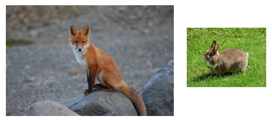
Foxes eat other animals (they are predators), including rabbits: rabbits are eaten by other animals (they are prey), including foxes, but rabbits eat only plants. Now let’s imagine an island that contains foxes and rabbits; there are no other animals for the foxes to eat and the rabbits have an unlimited supply of plants for food. There are no other animals or plants that can harm rabbits or foxes in any way. The science of how animals and plants interact with their environment, including other animals and plants, is called ecology. And a system in which animals and plants coexist with their environment is called an ecosystem. So, our island is a simple model for an ecosystem.
Let’s suppose that at time t, the number of rabbits in our ecosystem is R and the number of foxes is F. Then the rate of increase in the number of rabbits, dR/dt, is proportional to R (see post 18.15). But, at the same time the rate of decrease in the number of rabbits, -dR/dt, is proportional to F (more foxes to eat rabbits) and R (the greater the value of R the more rabbits can be eaten). So the overall increase in the rabbit population is
dR/dt = AR – BFR (1a)
where A and B are constants.
Now let’s think about the number of foxes. The rate of increase in the number of foxes, dF/dt, depends on how much food they eat, BFR (see previous paragraph) but the rate of decrease of the fox population, -dF/dt, is proportional to F (because the more foxes there are the more of them need to share the available food. So overall the increase in the fox population is
dF/dt = BFR – CF (1b)
where C is a constant.
Equations 1a and 1b are examples of coupled differential equations because we cannot solve one without reference to the other. These two coupled differential equations, that provide a simple model for the populations of predators and prey are called the Lotka-Volterra equations. Alfred Lotka (1880-1949) was born in the Ukraine but moved to England, where he obtained his undergraduate degree from the University of Birmingham. He then moved to the USA where he did research in mathematical biology and on using statistical ideas from physics (see posts 16.38 and 20.26) to investigate the economy. His research ideas were well ahead of his time. Initially he worked as a patent examiner (like Einstein) but later became statistician to an insurance company. He turned down offers of many university positions, perhaps because he could earn more at the insurance company! Vito Volterra (1860-1940) was an Italian mathematician with a much more conventional background – although he lost his job at the university for opposing the fascist leader Benito Mussolini. Lotka and Volterra developed equations 1a and 1b independently at about the same time.
Now let’s suppose that R and F remain constant, in other words dR/dt = dF/dt = 0. Then, from equations 1a and 1b
AR’ – BR’F’ = 0 (2a)
and
BF’R’ – CF’ = 0 (2b)
where R’ and F’ are the steady state (constant) values of R and F. Adding equations 2a and 2b gives
AR’ – CF’ = 0 or F’ = AR’/C. (3)
From equations 2a and 3
F’(C – CBF’/A) = 0.
If F’ ≠ 0 (in other words, there is a non-zero number of foxes)
C – CBF’/A = 0 or F’ = A/B. (4)
And, from equations 3 and 4
R’ = F’C/A = C/B. (5)
Is there any reason to believe that, at the beginning, the number of foxes and rabbits on our island was related to the constants in the Lotka-Volterra equation by equations 4 and 5? No! So, these results may be interesting but they’re not very important.
More general solutions of the Lotka-Volterra equations can become very complicated. So I want to make a simple assumption and look at its consequences. Let’s suppose that the number of rabbits differs from R’ by only a small number r. And that the number of foxes differs from F’ by only a small number f. Then the number of rabbits and foxes oscillates and repeats itself in a time period of
T = 2π/(AC)1/2 (7)
as explained in appendix 1. Then the population of rabbits oscillates as shown in the picture below. In this graph the rabbit population is expressed as a fraction of R’. To plot the graph, I used values of A = 1 year-1 and C = 1 year-1; also, I decided the maximum value for r would be r0 = 0.1R’. There are no special reasons for these values – I simply needed some reasonable numbers to plot a graph. For more details about the graph, see appendix 2.
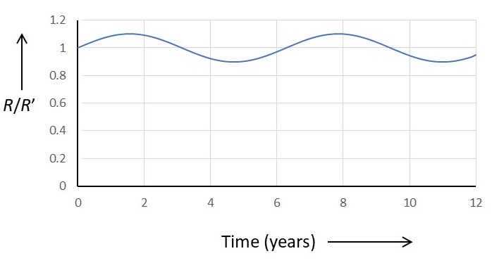
If you were to observe the rabbit population on the island during time period 2 > t < 4 years, you might be alarmed about the decline in the rabbit population. What has gone wrong for the number of rabbits to decrease in this way? The answer is that nothing has gone wrong. The decrease is a natural consequence of the oscillatory rabbit population. The fox population is also oscillatory – I hope I’ve given enough information (in the appendices) for you to plot a graph, like the one above, for foxes.
Of course, real ecosystems are much more complicated than this simple model. But the model does show that populations can be stable even if their numbers oscillate – in much the same way that a moving object has dynamic stability but is not in equilibrium (see post 22.9). But we must be a bit careful. Our model assumes that R is never very different from R’ (because we assume that r is small compared with R’). But a sustained fall in R to well below R’ is a cause for concern.
As increasing numbers of people are concerned about our environment the word “ecology” is increasingly used to mean caring for the world we live in and an “ecologist” can simply mean someone who is concerned for our environment. I believe it these concerns are very important. But we shouldn’t believe that an ecosystem should remain static. Indeed, a healthy ecosystem may be self-correcting, as suggested by the Gaïa hypothesis of the British scientist James Lovelock (1919-2022). However, if an ecosystem is subjected to serious abuse, it is unlikely to be able to correct itself. As an extreme example if most of the world’s water sources were contaminated by high concentrations of toxic waste, everything would die. The result (universal death) might remain stable but it wouldn’t be what we normally consider an ecosystem.
Related posts
16.42 Keep it simple
16.8 Predictions
Follow-up posts
Appendix 1
Oscillatory solution to the Lotka-Volterra equations
Let R = R’ + r (r is much less than R’) and F = F’ + f (f is much less than F’).
Then equations 1a and 1b become
d(R’+r)/dt = A(R’ + r) – B(F’ + f)(R’ + r) (7a)
d(F’ + f)/dt = B(F’ + f)(R’ + r) – C(F’ + f) (7b)
Noting that F’ is a constant, equation 7b becomes
df/dt = (F’ + f)[ B(R’ + r) – C].
Now I’m going to substitute expressions for F’ and R’ from equations 4 and 5 into this result, to give
df/dt = AC/B + Ar – AC/B + Bf(C/B) –Cf = Ar. (8)
The derivation above assumes that fr is so small that it is negligible.
We now have an expression for df/dt that depends only on the number of rabbits. So let’s return to equation 7a and look at the rabbit population. Noting that R’ is a constant and assuming that fr is negligible, this equation becomes
dr/dt = A(R’ + r)– B(R’F’ + R’f + rF’).
Now we’re going to get rid of a lot of constants by differentiating, with respect to time, once more to give
d2r/dt2 = A(dr/dt) – BR’(df/dt) – BF’(dr/dt)
and then substitute expressions for F’ and R’ from equations 4 and 5 into this result, to give
d2r/dt2 = A(dr/dt) – (BC/B)(df/dt) – (BA/B)(dr/dt) = – C(df/dt). (9)
From equations 8 and 9
d2r/dt2 = – ACr. (10)
Equation 9 is the equation of a simple harmonic oscillator whose time period is given by equation 7.
Appendix 2
Plotting a graph of the rabbit population against time
If the rabbit population oscillates about R’ and r is initially zero, following what we know about simple harmonic oscillators, we can write that
r = r0sinωt = r0sin(2π/T)t
where r0 is the maximum value of r, ω is the angular frequency of the oscillation and T is its time period.
Substituting for T from equation 6 gives
r = r0sin([AB]1/2t).
Remember that R = R’ + r.
