Before you read this, I suggest you read post 22.12.

In post 22.12, we saw that, in the microscope, the first stage of image formation was formation of a diffraction pattern in a plane that I have labelled the diffraction plane. Waves then continued to form an image, so that the image of point A appears at A’. In the picture above, I use ray-tracing to show how a ray scattered by A arrives at A’; the first stage is that it is scattered through the angle φ.
When we are thinking about diffraction we often use the modulus of the scattering vector
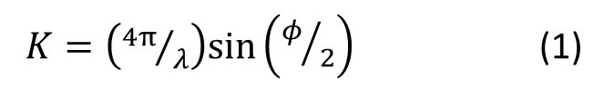
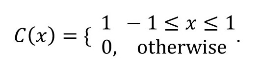
instead of the scattering angle φ (see post 19.20). Here λ is the wavelength of the scattered waves. In post 22.12 we considered scattering a simple one-dimensional object of uniform width 2 units and height 1 unit. Then the wave scattered in the K-direction could be represented, in amplitude and phase, by

where x represents a distance in the one-dimensional object. But there is a problem. If we wanted to compute an image, instead of creating it optically, we would need to calculate the integral

If you are puzzled by this, it’s just equation 5 of post 22.12 when.
(see post 22.11) so that C(x) has a centre of symmetry with the result that ψ(K) is not complex (compare with equation 5 of post 22.12, noting that equation 3 is its inverse).
But, in the microscope, we cannot use an infinite range of K values (that is an infinite range of φ values) to form an image. Why not? Because the picture shows that, in a microscope φ must be less than 90o if a ray is to pass through the objective.
Now remember that the image is formed by adding waves that have passed through the diffraction plane. Equation 2 shows that, in our simple example, these are all sine waves. In post 18.14 we saw that the fundamental wave, when
Kx = 2π (4)
defines the outline of the image and that higher K values (corresponding to higher spatial frequencies, in this case defining the sharp outline of the object in the image) create detail. If you don’t understand equation 4, remember that we need a complete cycle of the sine wave (360o or 2π radians) of equation 2 to contribute to the image.
From equations 1 and 4

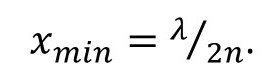
To see as much detail as possible in the image, we want x to be as small as possible – so we want sin(φ/2) to be as large as possible. The largest possible value for the sine of any angle is 1. So, the smallest object we can see in the microscope is

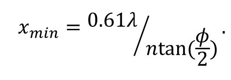
We call the value of xmin the resolution of the microscope. Sometimes you will see this equation modified to allow for a medium of refractive index n between the object and the objective. Then equation 6 is modified to give
Many textbooks calculate the resolution of the microscope by considered light scattered by a circular object. Then
So, the exact result depends on the form of the object. I didn’t choose a circular object because the mathematics is more difficult.
The important point is that the smallest object we can see in a microscope is about the same size of the wavelength of the waves we use to form the image. Since light has a wavelength of around 500 nm, we can use a light microscope to see bacteria (dimensions around 1 μm) but not most viruses (dimensions usually less than 200 nm).
If we want to see viruses, we can use an electron microscope. When electrons are accelerated through a potential difference of about 100 kV, they have a wavelength of about 3 pm. (For information on electron and neutron waves see post 19.25.) In an electron microscope, electrons are focussed by electromagnets. But these magnets cannot be made to focus electrons as well as we might wish. So, the resolution of an electron microscope is much less than 3 pm but is adequate to see viruses.
Suppose we want to see the positions of atoms in a molecule that are about 0.1 nm apart. The resolution of the electron microscope is too poor to see them. But we can obtain x-rays and neutrons with a wavelength of about 0.1 nm. Unfortunately, there are no lenses available for x-rays of this wavelength or for neutrons. So, to investigate the positions of atoms in molecules we must content ourselves with obtaining information from the diffraction pattern – as in the technique of x-ray diffraction.
Related posts
22.12 Diffraction, image formation and Fourier transforms
22.11 The microscope
19.20 Diffraction
18.14 Wave shapes
Follow-up posts
