In post 16.29, we saw that the lowest energy levels in an atom are conventionally labelled, in order of increasing energy, 1s, 2s and 2p. There are three 2p levels that all correspond to the same energy; they are denoted 2p_x, 2p_y, and 2p_z. Electrons occupy these energy levels according to the principles explained in post 16.29. For example, let’s remind ourselves of the energy levels occupied by electron in a carbon atom. A carbon atom has six electrons. Each energy level can accommodate a maximum of two electrons, provided they have opposite spin (see also post 20.27). Then we can represent the occupancy of electron energy levels in a carbon atom as 1s², 2s², 2p_x¹, 2p_y¹, where the superscript numbers show the number of electrons in each energy level. This result is shown in a picture in post 16.29. Note that one electron occupies 2p_x and another 2p_y; this enables the system to maximise the total electron spin – we won’t concern ourselves here about why this is. Why do the electrons occupy 2p_x and 2p_y, rather than 2p_y and 2p_z or 2p_x and 2p_z? It doesn’t matter because, as we shall soon see, the labelling of 2p_x, 2p_y, and 2p_z is arbitrary because it depends on how we define our coordinate system.

Electron energy levels in atoms can be measured by measuring the energies of the photon that they absorb. If we want to calculate these energies from first principles, we need to solve Schrödinger’s equation for an electron in an atom. In post 19.28, I give a much simpler example of solving this equation. The first stage is to obtain a wave function, ψ that can then be used to calculate an energy level. ψ provides information about position – in this case the position of an electron in an atom. But it can’t tell us the exact position – this would violate Heisenberg’s uncertainty principle. In post 19.29, we saw that there were several possible interpretations of ψ, but I am going to use the interpretation of post 19.28. Note that ψ can be a complex number and we can represent its complex conjugate by ψ*. Then the value of ψψ* at a point in space represents the probability of finding an electron at that point.

You don’t need to read this paragraph to understand this post – so you may want to ignore it. Calculation of ψψ* destroys all phase information about the electron wave – see posts 18.16 and 18.17. We could also think of ψψ* as a measure of the energy transmitted by an electron wave of amplitude ψ – see post 19.8. When we detect a wave, we measure its energy, as described in post 19.8. So, we could think of the process of detecting the electron wave as reducing the information carried by ψ to a probability. This loss of information on observation is sometimes called collapse of the wave function.

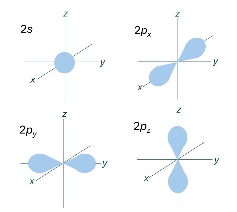
A region of space that has a high probability (typically 95%) of containing an electron associated with an atom is called an atomic orbital. The orbital associated with the 1s level is a sphere whose centre is at the atomic nucleus. In the picture, I have defined an orthogonal Cartesian coordinate system whose centre is at the atomic nucleus. The picture shows atomic orbitals associated with 2s, 2p_x, 2p_y, and 2p_z energy levels. The 1s atomic orbital is a sphere. But the others are less symmetrical and have only cylindrical symmetry about the axis that gives them their name – this means that, for example, that the shape of the 2p_z orbital is unchanged by rotation about the z-axis that it surrounds. A more rigorous explanation of cylindrical symmetry is given in the appendix.

In the next posts, we will use the shapes of atomic orbitals to understand more about molecules.

Related posts

19.29 Interpreting quantum mechanics
19.28 Solving Schrödinger’s equation
19.27 Schrödinger’s equation
19.26 Heisenberg’s uncertainty principle
19.25 Wave-particle duality
19.24 Electron waves
16.31 Electrons in molecules
16.29 Electrons in atoms

Follow-up posts

25.1 Hybrid orbitals
25.8 The sphere

Appendix – Cylindrical symmetry

I am going to use a cylindrical polar coordinate system to give a more rigorous explanation of cylindrical symmetry.

I defined a two-dimensional polar coordinate system (r, θ) in post 21.3. In post 22.15, I introduced a second angle, φ, to define a position in a three-dimensional space using a spherical polar coordinate system (r, θ, φ).

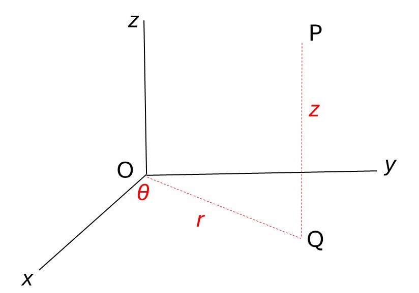
Now I am going to define a position in a three-dimensional space using the cylindrical polar coordinate system (r, θ, z) shown in the picture above. Here the position of the point P is defined by a distance, r (that lies in the xy plane of an orthogonal Cartesian coordinate system), an angle, θ, (measured with respect to the x-axis) and a distance z (identical to z in the Cartesian system). So, a spherical polar coordinate system would define the position of P by a distance and two angles; a cylindrical polar coordinate system defines it by two distances and an angle. I used a cylindrical polar coordinate system, without giving it this name, implicitly in post 21.6 to describe the geometry of the helix.

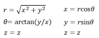
To convert between cylindrical polar coordinates and orthogonal Cartesian coordinates, we use Pythagoras’ theorem and simple trigonometry to derive the equations below (arctan is defined in an earlier post).

Now let’s suppose f(r, θ, z) is a function of r, θ and z in a cylindrical polar coordinate system. If the form of f is independent of θ then f is cylindrically symmetrical about z. You might like to compare this with the concept of a spherically symmetrical function.