Before you read this, I suggest you read posts 16.21 and 18.10.

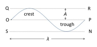
The picture shows a sinusoidal water wave (in blue) of amplitude A and wavelength λ (post 18.10) travelling along a straight channel at an instant in time, t. The wave is formed by water in the layer between the lines (that lie in planes in three dimensions) SN and QR that is raised (the crest of the wave) above or lowered (the trough of the wave) below, OP. Notice that OP would be the water level if there were no wave. Water below SN is not affected by the wave.

You can see that water in the crest of the wave has increased gravitational potential energy because it is raised above OP and water in the trough has negative potential energy, relative to OP (post 16.21). So, the average potential energy of a single wavelength is zero, relative to the resting water level, since a sinusoidal wave has the same mass of water in the peak and the trough.

What is the kinetic energy (post 16.21) of the wave? We can define an x-axis in the direction of propagation of the wave, along OP, and a y-axis that points upwards from it; the origin of this coordinate system is defined to be at O. Since water moves in the y-direction, the kinetic energy of the water in a single wavelength is

K = (1/2)m(dy/dt)²                 (1)

where m is the mass of water displaced and dy/dt is its speed (post 17.4). For a sinusoidal wave

y = Asin(ωt)                (2)

where ω is the angular frequency of the wave (equal to 2πf where f is the frequency, post 18.10). Differentiating equation 2 with respect to time gives

dy/dt = ωAcos(ωt)                 (3)

(see Appendix 1.2 of post 17.13). Substituting equation 3 into equation 1 gives

K = (1/2)mω²A²cos²(ωt).                 (4)

If the term cos²(ωt) looks a bit odd to you, it’s just the conventional wave of writing cos(ωt) multiplied by itself. Equation 4 gives the kinetic energy of the mass m of water at an instant in time t.

What is the average kinetic energy of this moving water during the time period, T, for a complete oscillation of the wave? We can write this as

K_av = (1/2)mω²A²<cos²(ωt)>_T.                  (5)

Here the <brackets>_T represent an average value over T. We only need to average over the cosine squared term, on the right-hand side of equation 5, because it is the only term that depends on time; m, ω and A are constants for a given wave.

It might not surprise you to know that <cos²(ωt)>_T is equal to ½ because the minimum value of the squared cosine of any angle is zero and the maximum value is 1 (see post 16.50). But this result isn’t as easy to prove. In the Appendix, I will demonstrate this result using a numerical method; I will not give a mathematical proof. (See Appendix 1 of post 16.50 to see why this isn’t a mathematical proof).

Knowing this result we can write equation 5 as

K_av = (1/4)mω²A² = mπ²f²A².                 (6)

If we design a mechanism that the wave can move, it is possible to convert its kinetic energy into useful work (post 16.21). The conventional way of doing this is for the mechanism to generate electrical energy (post 17.45).

Wave energy is one way of generating electrical energy. The rate at which this energy is generated is called wave power (post 16.23). Unfortunately, people often confuse “energy” and “power” when they’re talking about generation of electricity.

Another important point is that the energy of a wave is proportional to the square of its amplitude and the square of its frequency (equation 6). Because of this result, physicists couldn’t explain the photoelectric effect, in which light can make an electric current flow, until Einstein applied quantum theory to the problem.

Does this work for any wave shape? Yes – because any wave shape can be considered as the sum of sine and cosine waves (post 18.14) and a cosine wave is simply a sine wave with its phase increased by π/2 radians (post 18.10) – so what applies to a sine wave applies to any wave shape.

Related posts

18.17 Euler’s relation, oscillations and waves
18.14 Wave shapes – Fourier series
18.13 Sound
18.12 Vibrating strings
18.11 Motion in a circle, the simple harmonic oscillator and waves
18.6 The pendulum
16.21 Energy

Appendix

The average value of cos²(ωt) over the time period, T, is given by

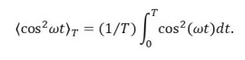
Why is this an average value? Because, I’m adding up all the values at infinitesimal values in time (post 17.19) and then dividing by the total time. We’re used to finding averages by adding up discrete vales; this generalises the idea to find the average value of a continuous function.

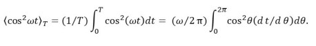
Now let’s define ϑ = ωt, so that t = ϑ/ω. This means that dt/dϑ = 1/ω (see Appendix 2 of post 17.4).

From the definitions of angular frequency and periodic time (post 17.12), ω = 2π/T.

So, when t = T, ϑ = ωt = ωT = ω(2π/ω) = 2π. Notice that ϑ is being measured in radians (post 17.11)

And, when t = 0, ϑ = ωt = 0.

Now we’ll put all this information into the equation at the beginning of the appendix, to give

And, finally,

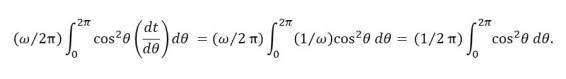
The final step arises because ω is a constant for a given wave and so can be taken outside the integral sign (see post 17.23).

If you like about things pictorially, you can see that we could have written the final step from the form of the cosine wave in post 16.50, and so saved ourselves a lot of algebra!

So, to find <cos²(ωt)>_T we have to evaluate the final integral between the limits 0 and 2π. But before we rush into doing this, let’s look at the graph below.

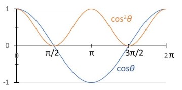
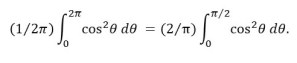
We can see that the average value of cos²ϑ in the range 0 to 2π radians is the same as its average value in the range 0 to π/2 radians. So

We can obtain an approximate value for this integral by considering the area under a graph of cos²ϑ, plotted against ϑ, as a series of thin strips of width Δϑ; we then add the strips, as described in post , so that

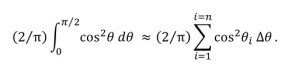
Here ϑ_i is the ith value of ϑ, where the first strip has i = 1 (ϑ₁ = 0 + Δϑ/2) and the final strip has strip has i = n (ϑ_n = π/2 – Δϑ/2).

Once we have chosen a value for n, Δϑ becomes (π/2)/n = π/2n. Then our summation becomes

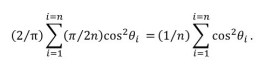
The final result makes it clear that we are calculating the average value of n strips. Using more imagination, we could have written this result without using any algebra!

In general, when we perform a numerical integration like this, the larger the value we choose for n, the better the approximation. But if you try this one (using Excel for example), you will find that you get a result of 0.5000 whatever value of n you choose. Below, I tabulate the results for 10 strips.

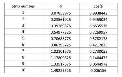
Adding the final column gives 5.000 and dividing by 10 gives 0.500.