Before you read this, I suggest you read posts 24.5 and 24.6.

In post 21.1 we saw that an electrical circuit that consists only of a capacitor discharging through an inductor is a simple harmonic oscillator in which the charge, Q, depends on time, t, according to the equation

Q = Q₀e^iωt                    (1)

(equation B4 in post 21.1). Here Q₀ is the initial charge stored by the capacitor, i is the square root of -1 and ω is the angular frequency of oscillation.

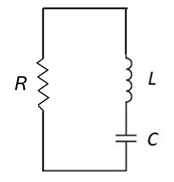
If we add a resistor, of resistance R, to the circuit, the oscillating charge will gradually dissipate energy (see dissipation in the index and post 21.1) so the system will become a damped simple harmonic oscillator, as described in post 24.6. This circuit is shown in the picture above.

Remember that current, I, is the derivative of the time-dependent charge with respect to t (see post 17.44), so that

I = dQ/dt.

Then the current in our circuit is given by

I = d(Q₀e^iωt)/dt = iωQ₀e^iωt = I₀e^iωt

(for information on differentiation, see post 22.10). If you’re worried that I₀ is a complex number, see appendix 1. This result means that the current, I, decays with time as described in post 24.6.

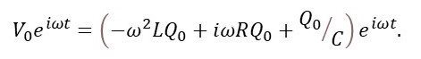
Now let’s suppose that we want to maintain an oscillating current our circuit, shown in the picture above. To achieve this result, we need to apply an oscillating potential difference, V, between the points A and B. The effect of this potential difference is to replace the energy dissipated by the resistor. According to post 24.5, this potential difference is given by

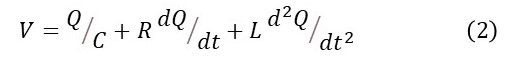
where V and Q depend on time. Assuming that C, R and L are constant, we have a linear second-order system. If we want V to drive the required oscillating current, it must be given by

V = V₀e^{i(ωt + ϕ)}.                    (3)

In general, there will be a phase difference, ϕ, between V and I (see posts 18.20 and 18.22) and, hence, between V and Q but they must all have the same value of ω if the oscillations are to be maintained with the required frequency.

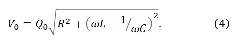
In appendix 2, I show that the required oscillating current will be maintained if

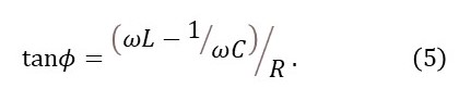
Now let’s define the phase of the oscillations to be zero when the capacitor is fully charged. Then, according to appendix 2, the phase of V is given by

Equations 3, 4 and 5 provide all the information we need to drive our oscillator.

The same ideas apply to a mechanical harmonic oscillator (appendix 3) and equations 4 and 5 are linked to the concept of resonance (appendix 4).

Related posts

24.6 Damped simple harmonic oscillator
24.5 Linear second-order systems
22.18 Coupled oscillators
21.1 An electrical simple harmonic oscillator
18.23 Frequency response and resonance in electrical systems
18.11 Motion in a circle, the simple harmonic oscillator and waves
18.8 Natural frequency and resonance
18.6 The pendulum: a simple harmonic oscillator

Appendix 1

How can I₀ be an imaginary number?

We have defined

I₀ = iωQ₀.

To answer the question, let’s think about

I = iωQ₀e^iωt = iωQ₀(cosωt + isinωt) = ωQ₀(icosωt – sinωt).

To obtain this result, I have used Euler’s relation. The real part of this result is a sinusoidal oscillation (when I is plotted against t, the result is a sine wave) that is initially zero and so represents the current in the circuit just before the capacitor discharges. So

I =  ωQ₀sinωt = I₀sinωt.

This means that it is the real part of the complex I₀ that describes the physical system.

See also appendix 2 of post 21.1.

Appendix 2

Derivation of equations 4 and 5

From equation 1,

dQ/dt = iωQ₀e^iωt   and   d²Q/dt² = –ω²Q₀e^iωt                    (6)

From equations 1, 2 and 6

So that

This means that V₀ is the complex number

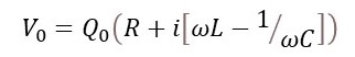
that is characterised by a modulus, given by equation 4 and a phase, with respect to the phase of I, given by equation 5. For more details, see post 18.17.

Appendix 3

Mechanical system

In a mechanical oscillator the displacement, x, of an object of mass m is driven by a time-dependent force, F. The force replaces energy dissipated by drag, and a spring of stiffness k stores energy. For simplicity, I assume that the displacement is confined to a line so that

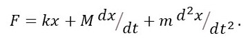
as described in post 18.24. So everything in this post applies to a mechanical system when k is analogous to 1/C, M is analogous to R and m is analogous to L; M(dx/dt) is the drag force (post 17.17). Then x is analogous to Q and F to V. As described in post 18.24, these analogies are not only mathematical – they also represent physical processes like energy storage (1/C and k), energy dissipation (R and M) and inertia (m and L).

Appendix 4

Resonance

Post 18.23 shows how equation 4 leads to the concept of resonance and how equation 5 leads to the concept of resonant frequency. The same ideas apply to mechanical resonance using the analogies described in appendix 3.