Before you read this, I suggest you read post 18.11

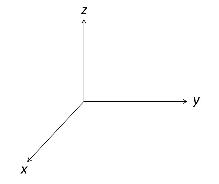
The picture below shows an orthogonal Cartesian coordinate system in which the z-axis is vertical. We are going to think of two pendulums: one oscillates in the xz plane and the other oscillates in the yz plane. For small oscillations, we can consider that the centre of gravity of the second pendulum moves in the x-direction and that for the first pendulum it moves in the y-direction; more details are given in posts 18.6 and 18.7. Then we can represent the motion of the two pendulums by

x = Asinωt   and   y =A’sin(ω’t + δ).

Here A and A’ are the amplitudes of the two oscillators, ω and ω’ are their angular frequencies and δ is the phase difference between them.

Now let’s suppose we have made a machine that couples the motions of the two pendulums. It will trace out a shape whose x and y coordinates are given by the equations above. These shapes are sometimes called Bowditch curves, after the American mathematician Nathaniel Bowditch (1773-1838). But they are usually called Lissajou’s figures or Lissajou’s curves after the French physicist Jules Lissajou (1822-1880) who investigated them in more detail.

The simplest way to obtain Lissajou’s figures experimentally is to use two electrical simple harmonic oscillators (see post 21.1) that create a sinusoidally varying voltage. The two voltages can then be plotted against each other using a device called an oscilloscope. Most descriptions of the oscilloscope (for example Oscilloscope – Wikipedia) will tell you that it plots a voltage against time but it can also be used to plot one voltage against another. But, to write this post, I have generated Lissajou’s figures with my computer.

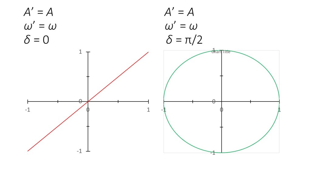
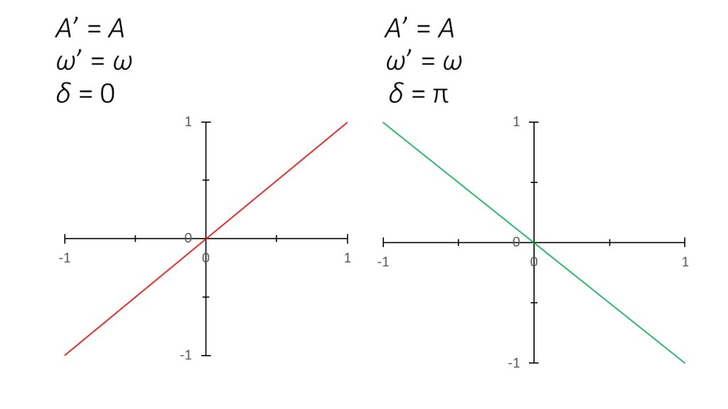
In the picture above, A = A’ and ω = ω’ and δ = π/2 (measuring the phase in radians). We can see that the resulting Lissajou’s figure is an ellipse. In the picture below, we can see that when δ = 0, the ellipse collapses into a straight line; when δ = π/2 it becomes a circle. I derive these results analytically in the appendix.

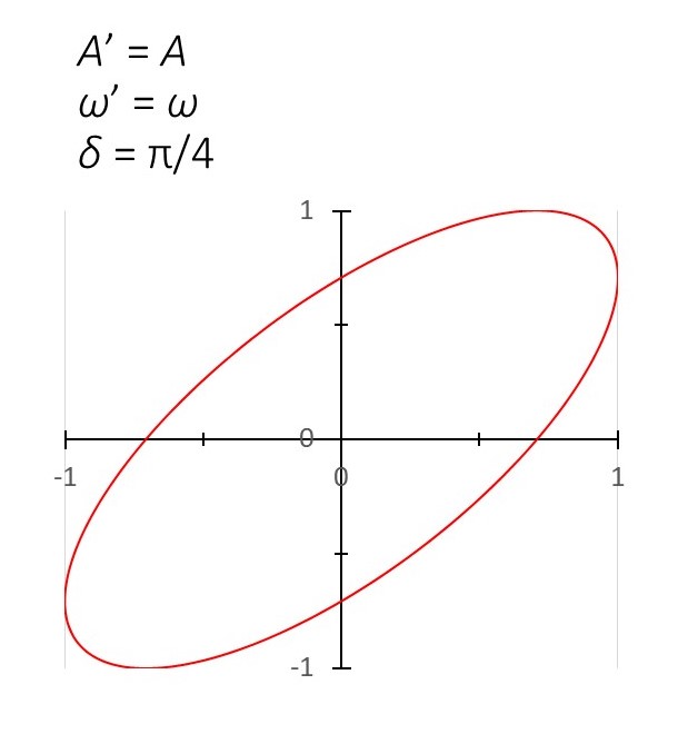
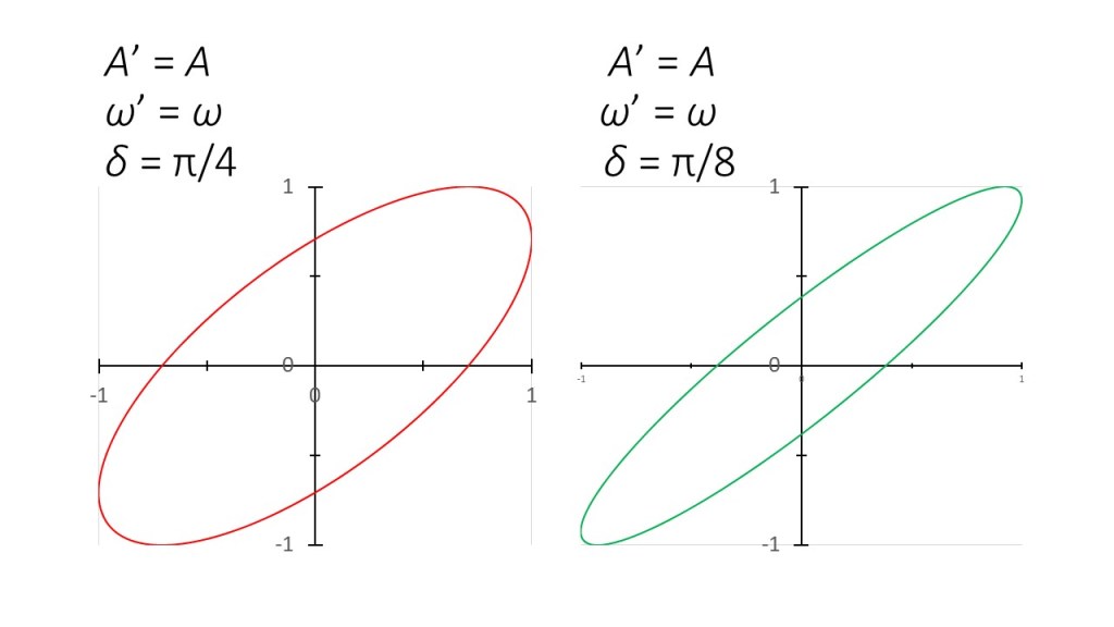
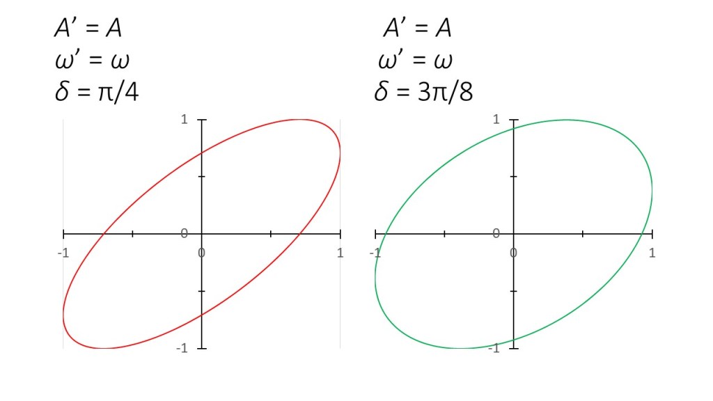
In the figures below we can see how making δ less than π/4 makes the ellipse narrower (more like a line) and making δ more than π/4 makes the ellipse wider (more like a circle).

And, in the pictures below, we can see that subtracting δ from π rotates a Lissajou’s figure through π radians.

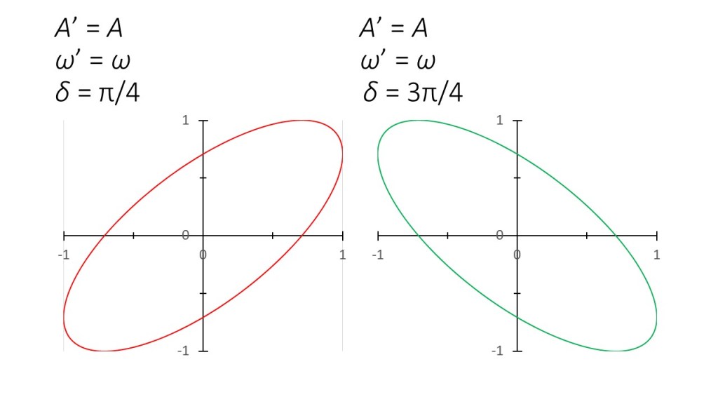
In conclusion, changing the value of δ changes the eccentricity of the ellipse and can rotate it by π radians. The eccentricity of an ellipse is the ratio of its major axis to its minor axis – defined in the picture below.

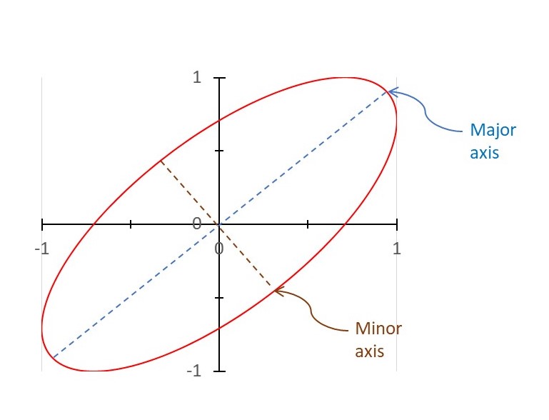
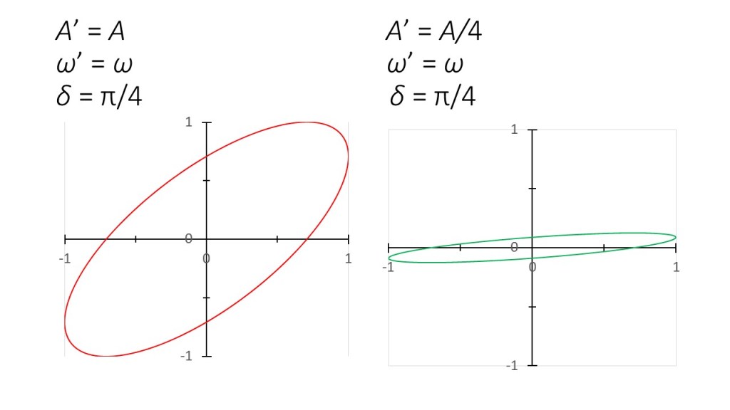
Changing the value of A changes the length of the minor axis and the orientation of the ellipse – see the picture below.

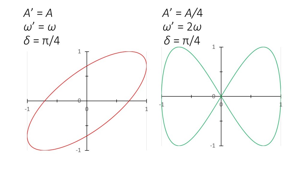
Now we’re going to investigate what happens when we change ω. In the picture below, you can see that the curve crosses itself when we double ω.

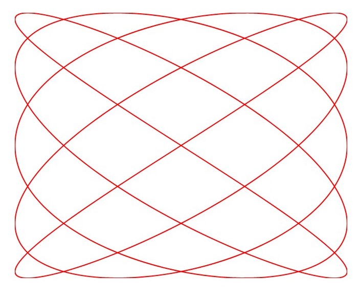
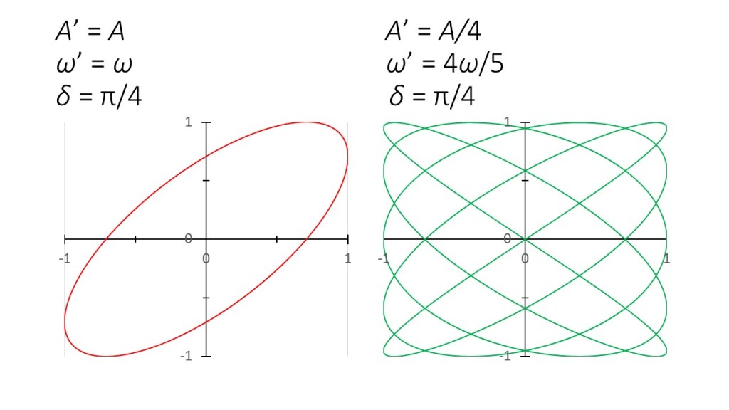
When we multiply ω by one integer and divide by another (neither integer is equal to 1), the curve crosses itself more times – as shown below.

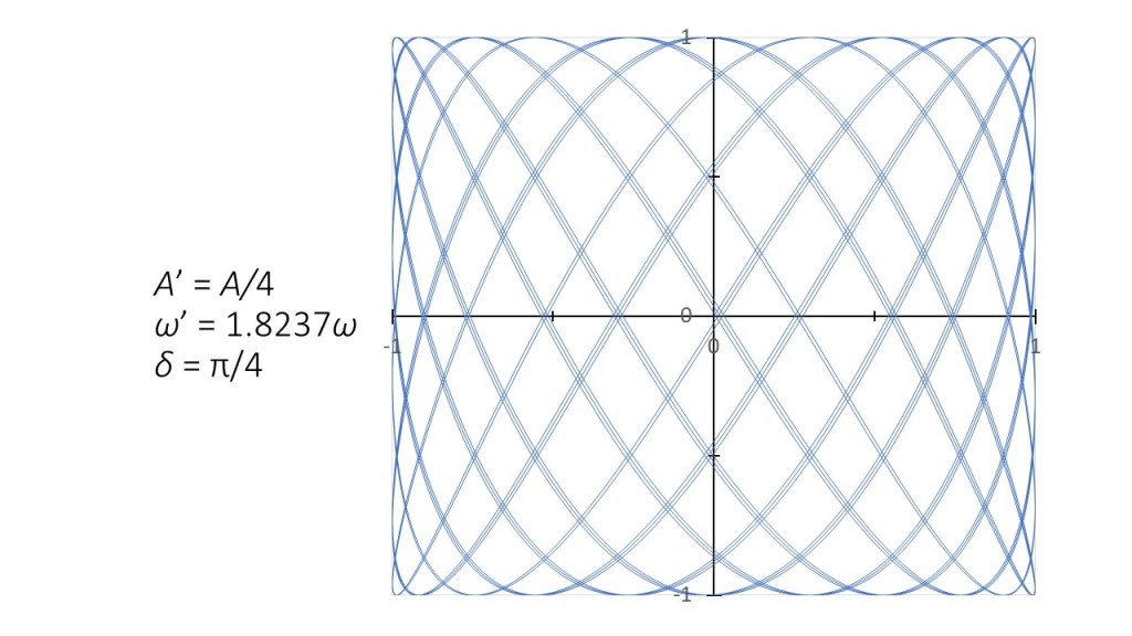
What happens when we multiply ω by an irrational number – one that cannot be expressed as the ratio of two numbers. If you look carefully at the picture below, you will see that the result is no longer a closed loop – the blue line follows a path that never re-joins itself.

What are Lissajou’s figures used for? According to some web pages, they are used to measure the frequency and phase difference between two electrical signals. The idea is that you can produce an oscillating voltage using a device called a signal generator. The frequency and phase of this signal can be varied and the Lissajou’s figure formed by plotting it against the signal that we want to know about. This seems to me to be a very complicated way of making these measurements. A friend of mine made measurements in this way – but that was over 50 years ago! He has never used Lissajou’s figures since!

So, why do I think Lissajou’s figures are interesting? I believe that they show how something as simple as coupling two simple harmonic oscillators can lead to a very wide range of, sometimes complicated, outcomes.

Related posts

22.8 The catenary
22.7 The caustic curve
21.6 The helix
21.5 Logarithmic spirals
21.3 Polar coordinates, circles and spirals
21.1 An electrical simple harmonic oscillator
19.17 Computer modelling – the simple harmonic oscillator
18.11 Motion in a circle, the simple harmonic oscillator and waves
18.7 The simple pendulum
18.6 The pendulum: a simple harmonic oscillator

Appendix

When A = A’ and ω = ω’, the equations at the beginning of the main text become

x = Asinωt   and   y =Asin(ωt + δ).

When δ = 0, y = x. This equation describes a straight line of slope 1 passing through the origin.

When δ = π/2,

y =Asin(ωt + π/2) = Acosωt

(see post 16.50). Then

x² + y² = A²sin²ωt + A²cos²ωt = A²

(see post 16.50) which is the equation of a circle of radius A (see post 21.3).