At the beginning of post 23.4, I described two routes to understanding x-ray crystallography. If you prefer the second, less mathematical, route – ignore this post!

Before you read this, I suggest you read post 23.8.

In post 22.14, we saw that the x-ray diffraction pattern of an object is given by the Fourier transform of its electron density, ρ(r). The electron density describes the distribution of electrons in the object as a function of r, the vector describing the position of a point in the object relative to some arbitrarily defined origin. Then we can represent the diffraction pattern of the object, both in amplitude and phase, by

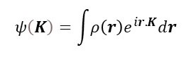
where the limits of integration are over the volume of the object (see post 17.19), e has an approximate value of 2.7183, i is the square root of -1 and K is the scattering vector that describes the direction of waves that make up the diffraction pattern (see post 22.23).

In post 23.8, we saw that the Fourier transform of a function provides coefficients a_n and b_n for the cosine waves and sine waves that we need to add together to construct the original function. So we can consider that Fourier transformation performs a frequency analysis of a function.

But, in post 23.8, we considered a function of time and calculated angular frequency, ω = 2πf where f is the frequency (conventionally measured in Hz). But, in x-ray diffraction, ρ(r) is a function of space so that Fourier transform tells us about frequencies in space – spatial frequency. So we can think of x-ray diffraction as an analogue method for spatial frequency analysis. Now K is the spatial equivalent of ω. Note that K is a vector because space is three-dimensional but ω is a scalar because time is one-dimensional. And in post 22.24, we saw that books about x-ray crystallography often consider a reciprocal lattice vector, S, instead of K, where S is the spatial equivalent of f.

The spatial equivalent of equation 1 of post 23.8 is

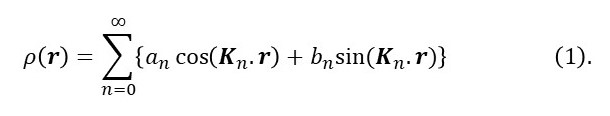
Here n is an integer; n = 1 corresponds to the fundamental frequency and higher values of n are the harmonics (see post 23.8); K_n.r is the dot product of two vectors giving a scalar result analogous to ω_nt.

In post 23.4 we saw that x-ray diffraction by a crystal is a common technique for determining the three-dimensional structure of molecules. So I am now going to concentrate on x-ray diffraction by a crystal. Then we need consider the electron density in a unit cell only, because an ideal crystal has a regularly repeating structure. This means that we can write ρ(r) as ρ(x, y, z) where x, y and z are fractional unit cell coordinates, as described in post 23.3. Also, post 23.3 shows that, for a crystal, we can write

K_n.r = 2π(hx + ky +lz)

where h, k and l are three integers called the Miller indices. Here we replace n by three integers because K and r are three-dimensional. I didn’t introduce them at the same time as equation 1 to keep my explanation as simple as possible. Now we can write equation 1 in the form

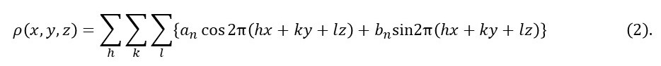
If you find it difficult to reconcile equation 2 with the final equation of post 23.3, remember Euler’s relation and that b_n can be negative and an imaginary number.

It appears that equation 2 lets us calculate the electron density in a unit cell. But there are two problems.

Problem 1. There is an experimental limit to the range of h, k and l values that we can observe (post 23.1). This limits the range of harmonics we can use to calculate ρ(x, y, z) so there is a limit to the level of detail we can observe. This is not usually a problem. But when determining the structure of a large molecule, like a protein, it may be necessary to combine the calculated ρ(x, y, z) with information from molecular modelling.

Problem 2. When we record an x-ray diffraction pattern, we cannot determine ψ(K); the best we can do is to determine ψ(K)ψ*(K) where ψ*(K) is the complex conjugate of ψ(K) (see post 22.14). This problem is called the phase problem in x-ray crystallography but can be solved by experimental or statistical methods (see post 23.4).

In previous posts I have developed all this material by comparing x-ray crystallography with image formation in the microscope and using the inverse Fourier transform. The purpose of this post is to develop these ideas using the Fourier series. It’s just a different way of looking at the same thing.

Related posts

18.14 Wave shapes
23.8 Frequency analysis
23.9 Discrete Fourier transform