Before you read this, I suggest you read post 23.8.
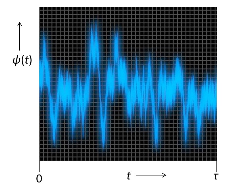
Let’s think about a wave or signal that looks like the picture above. It might be the result of an observation – for example, the electrical signal that results from recording a sound using a microphone. In this example we might want to know the relative proportion of the different frequencies (pitches) that characterise the quality of sound produced by a violin and that enable us to distinguish it from the sound made by a guitar (see post 18.12). We would need this information if we wanted to design a synthesizer that could mimic the sounds of different musical instruments. The same principles apply to voice recognition software and smartphone apps that recognise bird species from their songs.
In our example, we could think of the picture as an electrical potential, ψ(t) recorded as a function of time, t, from an initial time (defined as t = 0) until a final time (t = τ). Then, to distinguish musical instruments (or human voices or bird songs), the information we require is provided by a frequency analysis – as described in post 23.8. In post 23.8, we performed the frequency analysis by calculating the Fourier transform, F(ω), of ψ(t), defined by
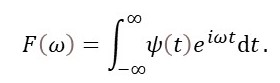
Here ω represents an angular frequency and i is the square root of -1.
But we now have two problems.
Problem 1. The Fourier transform has an infinite extent in time. But our signal is defined only in the range 0 ≤ t ≤ τ.
Problem 2. To calculate the Fourier transform, we to represent ψ(t) by a continuous mathematical function. But our signal does not resemble any recognisable function.
We can solve these problems by representing ψ(t) by a series of ψ values at N intervals in time separated by a time interval Δt, as shown in the picture below.
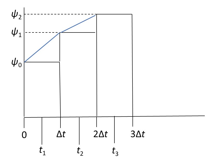
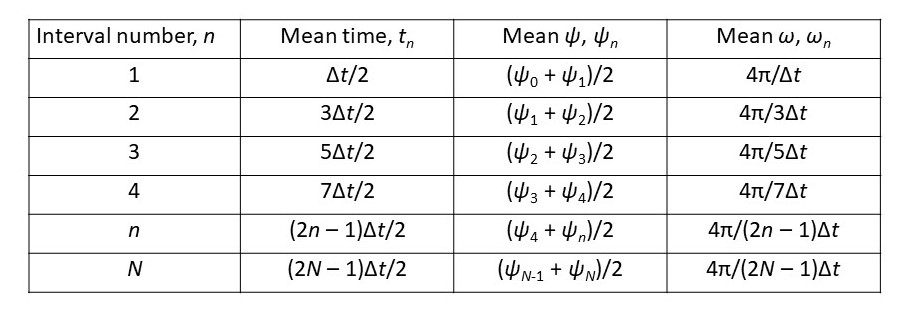
In this picture, the first interval (0 ≤ t ≤ Δt) occurs at a mean time of t1 = Δt/2 and is associated with a mean ψ value of ψ0 + ψ1. Here ψ0, ψ1, ψ2, ψ3 … are the values of ψ at times 0,Δt, ,2Δt, 3Δt … All this assumes that Δt is sufficiently small that all ψ values between ψn-1 and ψn lie on a straight line (we shall return to the value of Δt later). The table below shows the mean values of the time, ψ, and ω (2π/t) for each of the n time intervals.
To solve our problems, we represent the Fourier transform by a sum of discrete terms, representing discrete intervals in time. The result is
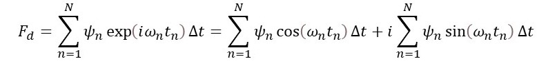
where the final step uses Euler’s relation and Fd(ω) is called the discrete Fourier transform. I have written ex in the form of exp(x) to make the equation easier to read. This is like the method we used to calculate the submerged volume of the hull of a ship in post 17.8.
According to post 23.8, we can write this result as
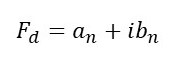
where an and bn are the coefficients of cos(ωntn) and sin(ωntn), respectively, that we can add together to form ψ(t).
We can see, from the table, that the lowest angular frequency is ωN; this is the fundamental frequency and ωN-1, ωN-2, ωN-3, … are possible harmonics (see post 18.12).
The values of (an/aN) are the relative contributions of cosine waves of angular frequency ωn to our signal; the values of (bn/bN) are the relative contributions of sine waves of angular frequency ωn to our signal. If the calculated value of (an/aN) is very small then that cosine wave makes a negligible contribution; if the calculated value of (bn/bN) is very small then that sine wave makes a negligible contribution.
But we need to be careful when n = 1, because ω1 corresponds to the sampling frequency. But, according to the Nyqvist criterion, the lowest frequency that we can detect is twice the sampling frequency. This means that our n = 1 results could be unreliable because of aliasing. So, our highest frequency harmonic, for which we have reliable information, corresponds to n = 2.
We can think of what I’ve written in the previous paragraph in a different way by thinking about the question, “How do we choose the value of Δt?”. Let’s suppose that the highest frequency harmonic we want to know about has an angular frequency ωmax. that corresponds to a time period of 2π/ωmax. According to the Nyqvist criterion, our minimum sampling frequency must be 2ωmax. which correspond to a time period of π/ωmax. This is the minimum value of Δt that we can use to reliably detect our required highest frequency harmonic.
Related posts
