In post 18.6, I defined a simple harmonic oscillator as a system that was constantly exchanging potential energy and kinetic energy while conserving their sum. I then used the idea of a simple pendulum as an example to illustrate how this works. In post 21.1, I showed how these ideas worked for an electrical simple harmonic oscillator – a circuit with no resistance in which a charged capacitor discharges through an inductor. I hoped that these specific examples introduced the idea as simply as possible – although the pendulum involved a lot of mathematical manipulation and its motion was derived more simply in post 18.7. Alternatively, we can investigate simple harmonic oscillations by computer modelling (see post 19.17).

Now I want to use the general idea of the simple harmonic oscillator, without considering any specific example. Most of the conclusions were reached in posts 18.6 and 18.11. I am going to consider that the oscillator has kinetic energy K, potential energy U n post 18.11.

The simple harmonic oscillator is a model for some real systems – it does not give an exact description of the motion of a pendulum or the discharge of a capacitor. Any real oscillator will gradually lose energy – a pendulum because of drag and a discharging capacitor because any real electrical circuit has some resistance. The behaviour of a damped harmonic oscillator is described in post 24.6. But the simple model provided by the simple harmonic oscillator helps us to understand the pendulum, the discharging capacitor and many other systems.

I am going to define the total energy of a mechanical system by

where K is the kinetic energy and U is the potential energy. If the system doesn’t lose or gain energy, the total energy remains constant so that

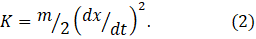
Here d/dt represents differentiation with respect to time. If the system is displaced by x, K is defined by

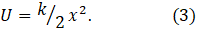
A mechanical system can store potential energy by compressing a spring and release the stored energy when the spring recoils; so that we can represent U by

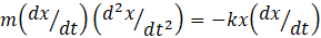
To see how this applies to gravitational potential energy, see appendix 1. In appendix 2 of post 20.3, we saw that it was a good approximation for low amplitude thermal oscillations of an atom in a solid that behaves as a simple harmonic oscillator. From equations 1, 2 and 3

We can calculate the derivatives in equation 4 using the methods described in post 22.10. But the derivative on the left-hand side is complicated, so I’ve explained how to do it in the appendix.

which simplifies to

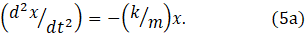
Equation 5a applies to displacement along a line; the equivalent result for rotational mechanical energy would be

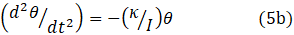
where θ represents angular displacement, κ represents rotational stiffness and I represents rotational inertia (see post 17.39). For an electrical oscillator, the corresponding result is

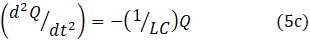
where Q represents charge, C represents capacitance and L represents inductance (see post 18.24).

I defined a simple harmonic oscillator in the first sentence of this post; an alternative (equivalent) definition, from equation 5, would be a system in which some quantity, ξ, varies according to

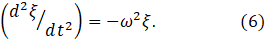
Here ω² is a constant for a given case; the reason for writing it in this form will become apparent later (if you haven’t already seen why). In post 24.5, we saw that equation 6 is a special case of a second-order linear system that doesn’t loose energy and has no external energy supplied to it.

Equation 6 has two trigonometric solutions

where ϕ and ψ are arbitrary phase angles. When   ϕ = 0   and   ψ = π/2   (or the other way round) the two equations are identical (see post 16.50 noting that here I am measuring angles in radians). ξ₀ is the maximum value of ξ (the amplitude of the oscillation). There is a third, exponential, solution

where i is the square root of -1 and χ is a phase. According to Euler’s relation, the solutions in equations 7a, 7b and 7c are linear combinations of each other, as expected for solutions of a differential equation (see post 19.10).

The solution we choose depends on the system we wish to describe. For example, if I wanted to describe the charge on a discharging capacitor, I would choose equation 7b with   ψ = 0,   so that at   t = 0   it had its maximum charge, Q₀. But if I wanted to consider the charge flowing in the circuit, I would choose equation 7a, with   ϕ = 0,   so that the initial charge in the circuit (when the capacitor was about to discharge) would be zero. I believe that phase angles are useful only when we want to relate one oscillation to another, as in post 22.18.

Now I want to think about what ω represents. Since the trigonometric solutions (equations 7a and 7b) repeat every 2π radians (post 16.50),   ω = 2π/t   represents the angular frequency of oscillation. Then the frequency of oscillation is given by   f = ω/2π   and the time period of oscillation is given by   T = 1/f.  

What I have written in the previous paragraph makes equation 5 very useful. If we can describe the motion of a system by this equation, we know that it is oscillatory and can simply write down its frequency. For example, when we find that the motion of a simple pendulum of length L in a gravitational field g is described by

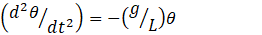
we know that its time period is

Related posts

24.7 Driven oscillator
24.6 Damped simple harmonic oscillator
22.18 Coupled oscillators
21.1 An electrical simple harmonic oscillator
19.17 Computer modelling – the simple harmonic oscillator
18.17 Euler’s relations, oscillations and waves
18.11 Motion in a circle, simple harmonic oscillator and waves
18.7 The simple pendulum
18.6 The pendulum: a simple harmonic oscillator

Appendix 1 To show the application of equation 3 to gravitational potential energy

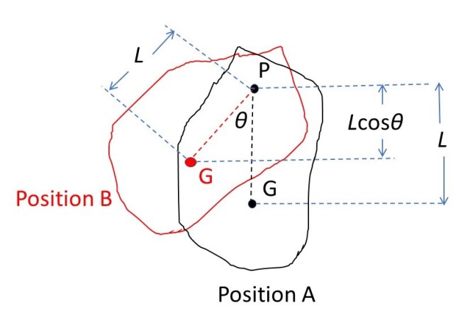
The picture above (from post 18.6) shows a pendulum, whose centre of gravity is at G, suspended from a point P; the distance from P to G is L. The height of, G’ (the position of G when the pendulum is displaced by an angle θ) above G, is given by   Lcosθ.   Then the potential energy of the pendulum is

The last step is justified in appendix 1 of post 18.6. Since θ is a small angle when measured in radians

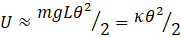
where κ is a constant. This result has the same form as equation 3.

For a pendulum that is a small object (of mass m) on the end of a string (of length L and negligible mass) the rotational inertia is given by

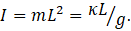
This result enables us to obtain equation 8 from equation 5b.

Appendix 2 To calculate the derivative on the left-hand side of equation 4

Let

Then