Before you read this, I suggest you read post 22.6.

In post 22.6, we looked at the path taken by a ray when it is reflected by a concave surface. We looked at two types of concave surface. In the first, a section of the surface was the arc of a circle; in the second, a section of the surface was a parabola. In the second case, all rays met the axis of the curve at a single focal point. But the first case was more complicated; in this post, we’ll investigate this case in more detail.

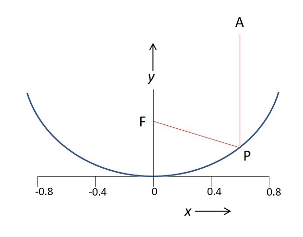
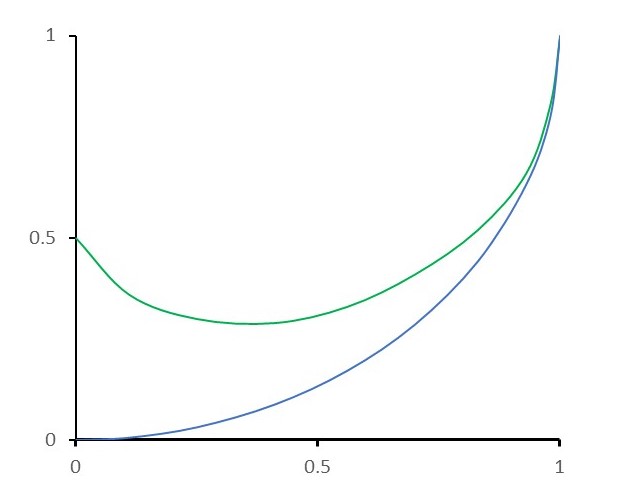
The picture above shows a section through a concave reflecting surface (in blue) whose axis defines the y-axis of a right-handed orthogonal Cartesian coordinate system whose origin is at the minimum of the curve – as in post 22.6. In this post, the section is the arc of a circle. We can generate a three-dimensional reflecting surface by rotation about the y-axis (as in post 22.6) but, later in this post, we shall see that there are other possible reflecting surfaces that can be generated from this arc. In the picture the line AP represents a ray, parallel to the y-axis, that meets the reflecting surface at P and is then reflected along the path PF. It will continue beyond F but I am interested in the distance, f, of F from the origin of the coordinate system. The direction of PF is defined by the laws of reflection, defined in post 22.4, applied to a concave surface, as in post 22.6. In this post I shall define the length of the radius of the arc, a, to be 1 unit; x and y values will be given in these same units. Then, from equation 3 of post 22.6, f is given by

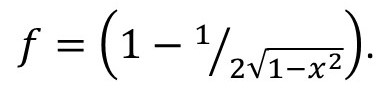
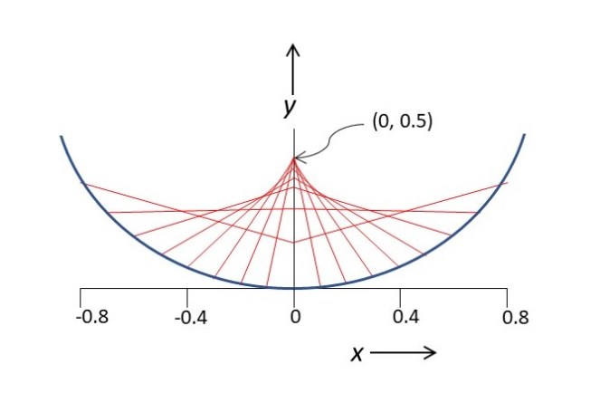
The picture above used this equation to show the position of F for different positions of P defined by x values in the range   -0.8 ≤ x ≤ 0.8.   For small values of x,   f ≈ 0.5,   as explained in post 22.6. But, as x increases, f decreases. When the rays reflected by different points cross, they define two curves – one on the left-hand side of the y-axis: the other on the right-hand side. To make this clearer, I have marked some crossing points with a green +, in the picture below.

The picture above shows (in green) the smooth curve through these points, on the right-hand side of the y-axis. This curve is called a caustic curve. Calculating this curve is not straightforward – if you want to know more about how I plotted it, see http://users.df.uba.ar/sgil/physics_paper_doc/papers_phys/ondas_optics/caustica1.pdf.

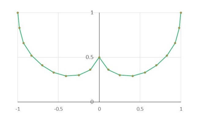
The picture above shows that when the right and left-hand halves of the caustic curve meet, the overall curve does not pass smoothly from one side to the other. When x = 0, there is a discontinuity, called a cusp, between the two halves.

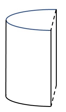
You can sometimes see the shape of a caustic on the surface of a drink when it is illuminated by a bright light. In this case the reflecting arc of the circle is not a section of a dish but a section through half a cylinder, as shown in the picture above. So look for a caustic curve on the surface of a drink when you’re outdoors on a sunny day.

Related posts

22.6 Reflection at concave surfaces
22.5 Total internal reflection
22.4 Reflection
22.1 Refraction at curved surfaces