Before you read this, I suggest you read post 21.17.
In post 21.17, we saw that beams can support a load because they are bent by it. I also gave some rules for calculating the deflection of some simple beams and the maximum stress in them. But I didn’t explain how these rules are derived.
This blog is supposed to encourage thinking about science – following rules that we don’t understand is not thinking! So, in this post, I want to explore the ideas behind these rules. But these ideas are not simple – so you may prefer to ignore this post, and the next, if you are not very interested in beams.
1 Radius of curvature
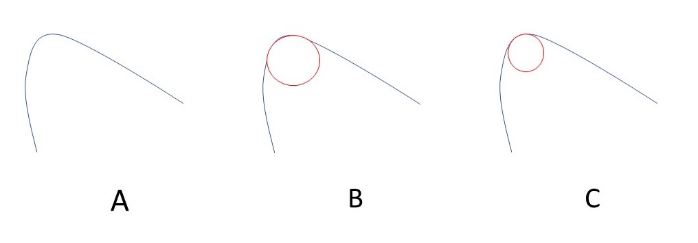
Part A of the picture above shows an asymmetrical curve. But, in part B, we can see that the top part of the curve closely fits an arc of a circle. When we chose a smaller region of the curve and make the circle smaller, in part C, the fit is even better. If we think the fit is sufficiently good for our purpose, we call the radius of the circle the radius of curvature for that part of the curve; the centre of the circle is its centre of curvature.
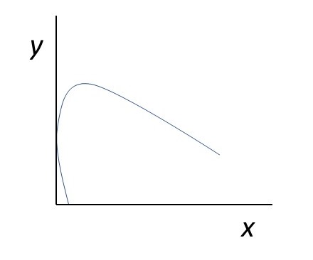
Now let’s think of the curve as being generated by plotting values of y against values of x, where y is a function of x, as in the picture above. We can now use our idea of radius of curvature, ρ, to define
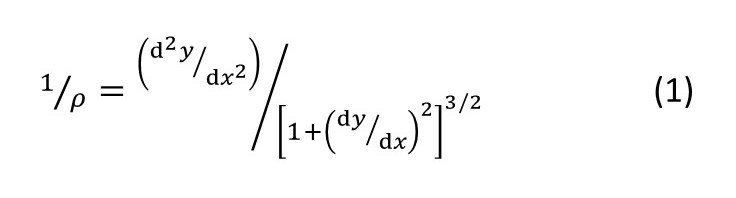
as explained in appendix 1. If the curvature is small (ρ is very large), by definition, dy/dx will be small so that (dy/dx)2 will be negligible. Then equation 1 becomes
1/ρ ≈ (d2y/dx2) (2).
Be careful, I have used y in a different way here than in post 21.17 that was also about beams.
2 Shape of a bent beam
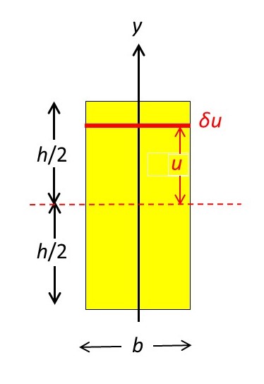
The picture above is a cross-section of a rectangular beam of height h and width b. The dotted red line passes through the centre of the beam and is perpendicular to its axis – so it lies in the plane of the neutral axis of the beam. We will define the y-axis to pass through the centre of the beam, perpendicular to its axis (that is, in the vertical direction) – as shown. When the beam bends, this cross-section will remain unchanged.
We are going to think about an infinitesimal element of the beam (shown in red in the picture above), a vertical distance u from the dotted red line, that has a height δu. So, this element has an infinitesimal area
δA = bδu (3).
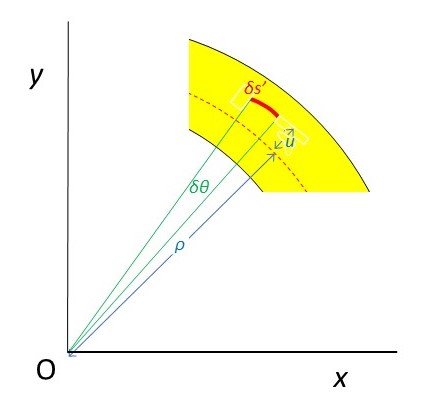
In the picture above, we are looking at a segment of the bent beam. The centre of curvature of this segment defines the origin, O, of a Cartesian coordinate system with the x-axis horizontal. In this plane, the bent red element has a length δs’. The green lines pass, from O to the ends of the red element; the angle between these ends is δθ (measured in radians). We define ρ as the radius of curvature of the neutral axis (dotted red line) of the beam between these green lines. Since we are considering an elemental segment of the bent beam, the curves between the green lines can be considered as arcs of a circle. Then
δs’ = (ρ + u)δθ (4).
Before the beam was bent, our element had the same length as an element on the neutral axis (whose length is unchanged by bending) which is
δs = ρδθ (5).
From equations 4 and 5, the tensile strain in our red element is
ε = [(ρ + u)δθ – ρδθ]/ρδθ = u/ρ.
(If our red element were on the other side of the neutral axis, the strain would be compressive.) The stress in our red element is then
σ = εE = Eu/ρ (6)
where E is the Young’s modulus of the material of the beam. So a force, perpendicular to the cross-section of the beam, is generated in the bent element; the modulus of this force is given by
δF = σδA =(Eu/ρ)bδu
from equations 3 and 6. This force is the restoring force generated in the stretched element. Noting that there will be no restoring force in the neutral axis, this force generates a torque of
δT = uδF = (Ebu/ρ)δu.
Then the total internal torque generated in a cross-section of the beam, through our bent segment, is
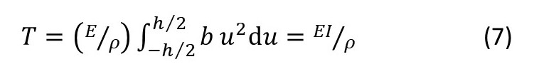
Here, I is the second moment of area of the cross-section. I have assumed that E and ρ are constant throughout the beam. More importantly, I have assumed that b remains constant throughout the cross-section, so that the cross-section is rectangular. However, if b were not constant (non-rectangular cross-section), I could simply replace the integral in equation 7 by more definite integrals (for a finite number of b values) or with a function that describes how b varies with u (for a continuous variation in b). The final conclusion (that T = EI/ρ) would remain unchanged. Books usually call T a bending moment because it’s a torque that tends to bend something.
From equations 1 and 7
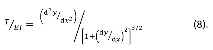
If we can calculate I and the restoring torque in a beam cross-section, and if we know E, we can, in principle, solve equation 8 to find how y depends on x. The result is the curve that describes the shape of a bent beam; this curve is called an elastica. Unfortunately, equation 8 can only be solved for very simple cases. Also, it will have more than one solution and, because it is a differential equation any linear combination of these solutions is also a solution.
3 Real beams
The bending in a real beam will be very slight. Then equation 2 becomes a good approximation to equation 1. As a result, we can replace equation 8 by
(d2y/dx2) = T/(EI) (9).
After calculating T and I, we can use equation 9 to find y at any value of x. In the next post, we shall see how we can use this result to calculate the deflection of a beam. We shall also see how we can use equations 6 and 9 to calculate the maximum stress in a beam.
Related posts
Follow-up posts
Appendix 1
The purpose of this appendix is to prove equation 1.
We will consider an elemental arc of length δs that subtends an elemental angle δθ at its centre of curvature. Then δs ≈ ρδθ so that in the limit δθ → 0,
1/ρ = dθ/ds. (A1).
If our curve is represented by y, a function of x, then θ is given by
θ = arctan(dy/dx) (A2)
where arctan is defined in post 17.2. This result recognises that the slope of y, at a given x value is given by the tangent of θ and dy/dx.
We can write
dθ/ds = (dθ/dx).(dx/ds) (A3)
as explained in appendix 1.2 of post 17.13.
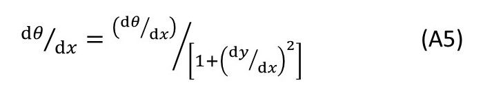
From equation A2
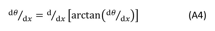
where u is a function of x, so that equation A4 becomes
We now need to find dx/ds to calculate ρ from equations A1, A4 and A5. If we approximate our elemental arc to a straight line, we can use Pythagoras’ theorem to write
(δs)2 ≈ (δx)2 + (δy)2.
Dividing both sides of this equation by (δx)2 and in the limit δϑ → 0 (when our approximation become exact), and then taking the square root of both sides of the result, gives
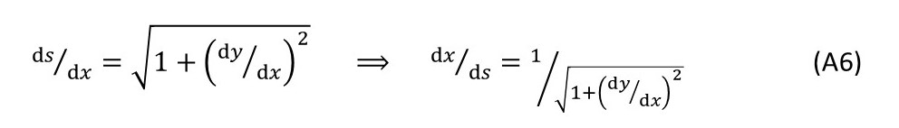
Substituting A5 and A6 into A1 gives us the required result.
Appendix 2
The purpose of this post is to prove that
where u is a function of x.
Let w =arctanx so that x = tanw (B1).
Then dx/dw = 1/cos2y (B2).
This result is proved in appendix 3. From the relationships between the sine, cosine and tangent of an angle (in the appendices of post 16.50)
cos2y = 1 – sin2y.
Dividing both sides of this equation by cos2y and noting that tany = siny/cosy gives
1 = (1/cos2y) – tan2y or 1/cos2y = 1 + tan2y (B3).
From equations B1, B2 and B3
dx/dw = (1 + x2) or dw/dx = 1/(1 + x2) (B4).
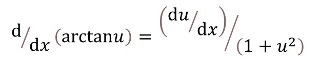
If w = arctanu then
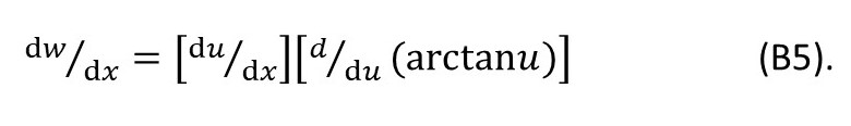
The definition of w in equation B1 and the result of equation B4 give the required result.
Appendix 3
The purpose of this appendix is to show that d(tanx)dx = 1/cos2x.
In appendix 1.3 of post 19.16, we saw that, if w = uv, where w, u and v are functions of x, that
dw/dx = u(dv/dx) + v(du/dx) (C1).
Since tanx = sinx/cosx, we can apply this result if u = sinx and v = (cosx)-1.
Then u(dv/dx) = (sinx)(cosx)-2(sinx) and v(du/dx) = (1/cosx) = (cosx) )(cosx)-2.
Then dw/dx = (sin2x + cos2x)/cos2x = 1/cos2x.
When I was at school, I was supposed to learn that if w = u/v then
But I didn’t because you can use equation C1, in the same way as I’ve used it here, instead. Why bother remembering things that you don’t need to know?
