In post 18.24 we saw that we could represent the displacement, x, of a mechanical system subjected to a time-dependent force, F by equation 1a. We also saw that the charge, Q, in an electrical circuit with a time-dependent potential difference across it could be represented by equation 1b. In both cases the variable, t, represents time. Since the values of F and V vary only with time, they are both functions of time and we could write them as F(t) and V(t), to make this dependence clear, but we don’t need to.

Using the analogy between translational and rotational mechanical systems (post 17.39) we could represent the angular displacement, θ, of a rotational system subject to a time-dependent torque, T, by equation 1c. Once again, T is a function of t.

In equation 1a, m represents the mass of an object subjected to the force, M(dx/dt) is the drag force acting on it and k represents the stiffness of the system. In equation 1b, L is the inductance of the circuit, R is its resistance and C its capacitance. All this is explained in post18.24. In equation 1c, I, D and κ are the rotational analogues of m, M and k, respectively, as explained in post 17.39. In general F, x, T and θ will be vectors. But here I am going to consider displacement along a line and rotation about a fixed axis, so I can represent them by scalars in this post.

Notice that equations 1b, c and d are all differential equations. Since the highest order of differentiation is two (in d²/dt²), they are second-order differential equations. Since the coefficients in these equations (for example, k, M and m in equation 1a) are all constants, these equations are linear second-order differential equations. (They would also be linear if the coefficients were functions of time only). The physical systems that they represent are called linear second-order systems.

In the remainder of this post, I want to think about systems that are not driven in any way. So I want to think about mechanical systems with no applied external force or torque and electrical systems with no applied potential difference. Then our differential equations become equations 2 below.

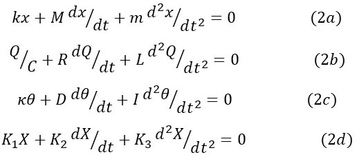
Equation 2d represents a general form for equation 2 in which X is any function of t only and K₁, K₂ and K₃ are constants.

Now we’re going to look at some special cases of equation 2d.

Case 1, K₃ = 0. This is the equation of exponential growth or exponential decay, as described in post 18.15. More details in appendix 1.

Case 2, K₂ = 0. This is the equation of a simple harmonic oscillator. More details in appendix 2.

Case 3, K₁ = 0. This is also the equation of exponential growth or exponential decay for the reasons given in appendix 3.

What does equation 2d represent when K₁, K₂ and K₃ are not equal to zero? This is the equation of a simple harmonic oscillator but with the extra term K₂(dX/dt). In post 18.24, we saw that this term represents the energy dissipated by a system. The process of dissipating energy in a mechanical system is called damping. So equation 2a and d are the equation of a damped simple harmonic oscillator. In post 21.1 we considered the simple harmonic oscillator to be an idealised model for a real system since any moving object will encounter some drag (even air has a non-zero viscosity) and any electrical circuit will have some resistance. So we could consider equation 2 to be a closer approximation to reality, although the energy dissipation term, K₂(dX/dt), will often be negligible.

I will solve the equation of the damped simple harmonic oscillator in the next post. And I haven’t yet considered the driven oscillator, for which F or V or T are non-zero – that’s a subject for a later post. For now, let’s just remember that equation 2 represents exponential growth and decay, simple harmonic oscillation and damped harmonic oscillation.

Related posts

22.18 Coupled oscillators
21.1 An electrical simple harmonic oscillator
19.17 Computer modelling – the simple harmonic oscillator
18.24 Analogies between electrical and mechanical systems
18.11 Motion in a circle, the simple harmonic oscillator and waves
18.7 The simple pendulum
18.6 The simple pendulum: a simple harmonic oscillator

Follow-up posts

24.6 Damped simple harmonic oscillator
24.8 Passive damping

Appendix 1

When K₃ = 0 equation 2d becomes

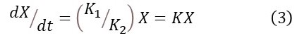
where K is a constant. In post 18.15, we considered equation 3 (equation 4 in post 18.15) to be one statement of the equation of exponential growth, when K is positive, and exponential decay, when K is negative.

Appendix 2

When K₂ = 0 equation 2d becomes

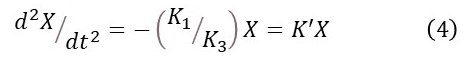
where K’ is a constant. In post 18.6, we considered a simple harmonic oscillator to be a system that was in the constant process of exchanging potential energy and kinetic energy. As a result, we saw that its motion was described by equation 4 (also equation 4 in post 18.6).

Appendix 3

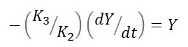
When K₁ = 0 equation 2d becomes

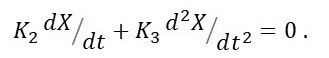
Integration with respect to t gives

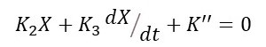
where K’’ is a constant of integration. Then

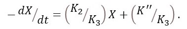
Let

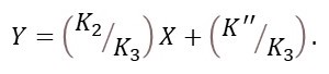
So that

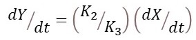
since K’’/K₃ is a constant. Now

So that

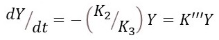
where K’’’ = –K₂/K₃ is a constant. This result has the same form as equation 3 and so represents exponential growth or decay.