I am going to calculate the Fourier transform of a Gaussian function because I want to use the result in a later post. I can define the Gaussian function, g(x) as an exponential function of the form

g(x) = exp(-ax²).

Here, exp(y) is another way of writing e^y where e a number with the approximate value 2.7183 (post 18.15).

In post 16.26 we defined the normal distribution, also called the Gaussian distribution, p(y), by

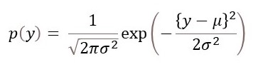
where μ is the mean of a set of y values and σ is their standard deviation. If we define   y = x + μ   and   σ² = 1/(2a),   we get the result that

p(y) = Cexp(-y²),

where C is a constant, for a given set of y values. So the normal distribution is a Gaussian function (multiplied by a constant) which is why it is often called the Gaussian distribution. (Since p represents a probability, the purpose of C is to ensure that p = 1 all possible y values, within the space they can occupy).

In the picture above (left-hand side), I compare g(x) for two different values of a. You can see that the width of g(x) decreases when a increases.

Previously, I have defined the Fourier transform of g(x) as

Then the Fourier transform of our Gaussian function would be

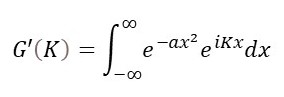
But in this post, I am going to investigate

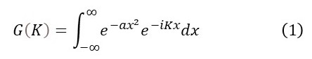
For the reasons discussed in Appendix 1; if you don’t want to read this appendix, the conclusion is that we can consider equation (1) as an equally valid definition of the Fourier transform of a Gaussian function. I have chosen this definition because it makes it easier to understand the calculation of the Fourier transform here.

The variable K defines the space we use to plot the Fourier transform (post 23.8) and i is the square root of -1 (post 18.16). Remember that, when we differentiate e^x, the result is e^x. And integration is the inverse of differentiation, so we expect that evaluation of the integral in equation 1 will give us an exponential function. In appendix 2, I show that evaluating this integral gives

There are many steps in this calculation and you may prefer to trust me that equation 1 leads to equation 2.

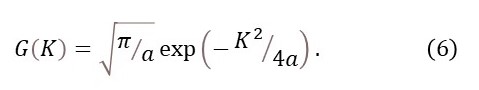
The picture (right-hand side) shows G(K) for the two a values used previously to plot g(x). Although increasing a makes g(x) narrower, it makes G(K) less narrow. This is what we might expect from the reciprocal relationship between dimensions in a function and its Fourier transform. For example, if we increase the distance between the points in a one-dimensional lattice, the distance between points in the reciprocal lattice (the Fourier transform of the lattice) decreases, as explained in post 22.22.

Follow-up posts

24.2 Thermal vibrations

Appendix 1

The purpose of this appendix is to comment on equation 1.

The last picture in post 22.12 shows that if we calculate the Fourier transform of a function and then calculate the inverse Fourier transform, we recover the original function. You can see this in the last picture of the post. I have ignored the factor of 2π since it is simply a scaling factor that does not change the form of the function. This result is retained if we define equation 3 to be the Fourier transform and equation 2 as its inverse.

According to post 18.11, changing the sign of the exponential function, in the definition of the Fourier transform, simply changes its phase. In post 18.10 we saw that the definition of the origin of phase is arbitrary so that we can consider either equation 2 or equation 3 (in post 22.12) to be the definition of the Fourier transform.

Appendix 2

The purpose of this appendix is to prove equation 2.

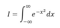
I start by defining

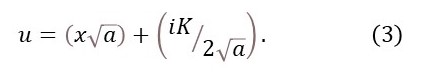
Then I can write

You can try deriving equation 4 from equations 1 and 3 or read appendix 2. The integral in equation 4 is called the Gaussian integral. In appendix 4, I show that this integral is given by

Then, from equations 4 and 5

Appendix 3

The purpose of this appendix is to prove equation 4.

From equation 3

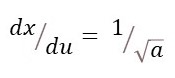
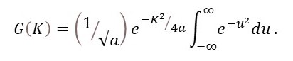
(see appendix 4 of post 17.4 noting that i² = -1) so that

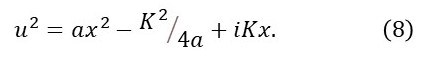
From equation 8,

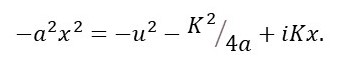
Then

 If you can’t follow the final step, see post 18.2.

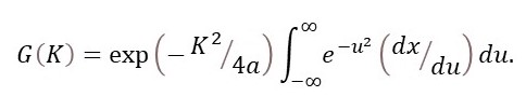
Substituting equations 7 and 8 into equation 1 gives

because the exponential term outside the integral sign is a constant and   e⁰ = 1.   Then

From equation 3,

so that

Appendix 4

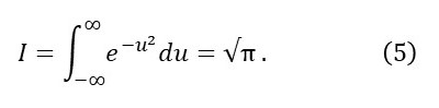
The purpose of this appendix is to prove equation 5.

Let

Then

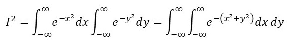
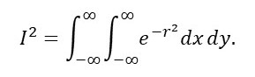
If we want to change to a polar coordinate system (to make the calculation easier) we note that the distance, r, in polar coordinates is given by   r² = x² + y² (see post 21.3).   Then

Changing the mapping of this integral, as described in post 22.16,

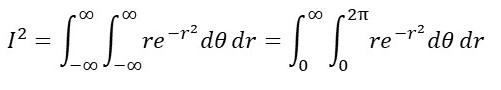
because r is completely defined in the range 0 to infinity and the angle, θ, in polar coordinates, is completely defined in the range 0 to 2π. Evaluating the first part of this integral gives

To calculate this integral, I’m going to define   v = r²,    so that dv/dr = 2r   and   r (1/2)(dv/dr) with the result that

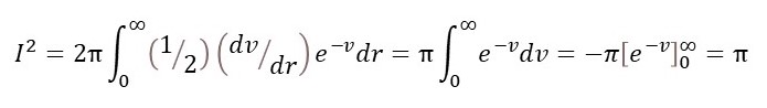
since   e⁰ = 1   and   e^∞ is itself infinity so that   e^∞ = 0 (see post 18.2). Taking square roots of the left and right-hand sides proves equation 5.