Before you read this, I suggest that you read posts 16.24 and 16.26.

In this post I want to explore how we make decisions based on experimental results.

Suppose two groups of rats, are identical in all respects, eat the same diet and live in identical conditions. However, one group is given a dietary supplement and the other isn’t.

At the end of a year, all rats that were given the supplement have a mean body mass of 0.420 kg (treated) but those that weren’t have a mean body mass of 0.404 kg (untreated). Can we decide that the supplement is associated with increased body mass? Because these numbers are means of a large range of values, we can’t make this decision confidently. We need more information.

In the graphs below I have plotted the number of rats with each body mass in the range 0.300 to 0.500 kg in steps of 0.005 kg, for the treated rats (red dots) and the untreated rats (blue dots). Although the mean body mass of the treated group is higher, there is a very wide spread of values and the results overlap with those from the untreated group.

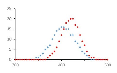
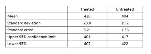
So, how are we to decide whether there is a difference? In the graph, the red dots all lie on the bell-shaped curve of a normal distribution (post 16.26) and so do all the blue dots. We can then calculate 95% confidence intervals, as described in posts 16.24 and 16.26. The stages of the calculation are shown in the table below.

Remember that an experiment can’t show that an idea is correct – it can only show that an idea is wrong (see post 16.3). So we start off with the null hypothesis that all the blue dots and all the red dots on the graph come from the same population of results; it’s called a “null hypothesis” because it supposes that there is no difference between the numbers represented by the blue dots and those represented by the red dots.

From the table we see that the 95% confidence interval for the untreated group does not overlap with the 95% confidence interval for the treated group. Therefore, the probability that our null hypothesis is false is at least 95%. Conventionally, we accept that this level of probability is evidence that there is an effect. We can say that there is a significant difference (p < 0.05) between the two groups; this means that there is a probability, p, of less than 0.05 (5%) that the two sets of numbers come from the same population. But be careful – we may need to use statistics to design something – then we need to be more than 95% confident that it won’t fail!

We can also calculate the probability that the numbers represented by the blue dots comes from the same population as the numbers represented by the red dots. We could do this using the properties of the normal distribution. But a more reliable method, especially for a small sample, is to use the t–test. The t-test assumes that our data are normally distributed, so we must check that they lie on the bell-shaped curve before we use this test. If you want to know how the t-test works, see https://en.wikipedia.org/wiki/Student%27s_t-test . However, it’s best to use established computer software to make statistical calculations, as explained in post 16.24. In Microsoft Excel, you can use the T.TEST function. But you could also use the online calculator at http://www.socscistatistics.com/tests/studentttest/ . For the results shown in the graph above, the probability that the red and blue dots come from the same population is only 3 × 10^-12 which is zero for all practical purposes. This is a much lower p value than you ever get from a real experiment – because I invented the results to show how decisions can be made from experimental results.

Suppose the results of an experiment are not normally distributed. What can we do? There are statistical tests that don’t assume a normal distribution – they are called non–parametric tests. They are less powerful at detecting significant differences than, for example, the t-test. This is because the t-test uses additional information about the data – that it is normally distributed. If the results from our two groups of rats had not been normally distributed, we could have compared them using a non-parametric test called the Mann-Whitney test (see https://en.wikipedia.org/wiki/Mann%E2%80%93Whitney_U_test ). You can’t use Microsoft Excel to do the Mann-Whitney test but there is an online calculator for calculating it at http://www.socscistatistics.com/tests/mannwhitney/ . Alternatively you can use specialist Open Source software: like GNU PSP (https://www.gnu.org/software/pspp/ ) or R (https://www.r-project.org/ ). R is very versatile but difficult to learn; I’ve never used PSP.

The important message is that we can’t trust that one experimental result is bigger than another without investigating whether the difference could have arisen by chance.

Related posts

16.26 Normal distribution
16.24 Accuracy and precision
16.8 Predictions
16.7 Writing numbers
16.3 Scientific proof

Follow-up post

20.4 Questionnaires
16.43 Test before you predict