Before you read this, I suggest you read post 25.13.
Electromagnetic induction arises when a current flows in a circuit when it is in a changing magnetic field (post 25.13). Faraday considered that the current flowed because an induced voltage caused charges in the circuit to move. Moving charges are an electrical current (post 17.44).
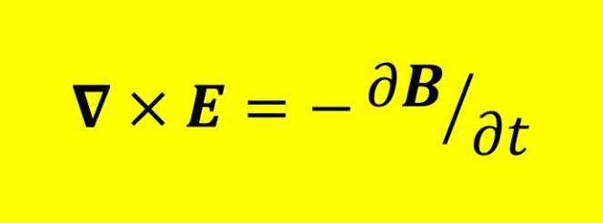
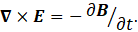
Maxwell realised that an equivalent explanation was that there was a variation in the electric field around the circuit, because charges can also be considered to be moved by an electric field (post 16.25). When Heaviside expressed Maxwell’s equations in vector notation, the result was the highlighted equation at the beginning of this post. This is the third of what we now call Maxwell’s equations. In this equation ∇ is the vector operator del, E is the induced electric field; ∇ × E represents the cross product of the vector operator ∇ and the vector E; ∂B/∂t represents the rate of change of the magnetic field, B, with respect to time. Note that ∂B/∂t is a partial derivative because B can also be a function of position. (I could have written ∇ × E as curlE). In post 16.25, we saw that a magnetic field was the result of electrical current; this was discovered by the French physicist André-Marie Ampère (1775-1836) whose name is used for the unit of electrical current – the amp. Maxwell’s third equation provides further information on the relationship between electric and magnetic fields.
In appendix 1, I show how Maxwell’s third equation can be derived from equation 1 of post 25.13. Now I am going to look at some of the implications.
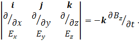
According to post 20.34, we can express the cross product in the equation by the determinant in equation 1.
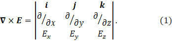
Here i, j and k are the unit vectors defining the x, y and z axes of an orthogonal Cartesian coordinate system. Ex, Ey and Ez are the x, y and z components, respectively, of E. So we could write Maxwell’s third equation as
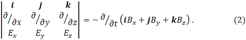
Here Bx, By and Bz are the x, y and z components, respectively, of B.
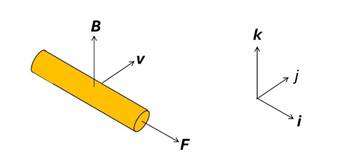
To see how this works let’s think of a one-dimensional magnetic field that defines the k direction (the z-axis), as in the picture above that is copied from post 25.13, where it is explained in more detail. Then Bx = By = 0 so that
The only way this can be true is if
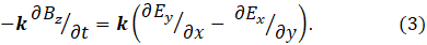
In the picture, a segment of conductor moves in the j (y-axis) direction with a velocity v. It does not move in the i (x-axis) direction. Since the only change is in the y-axis direction, only the second partial derivative in equation 3 is relevant to our segment. So the result is that an electric field exists in the x-axis direction, that is along the length of the conducting segment; as a result, a current flows in the segment.
Faraday’s original experiments on electromagnetism involved moving a conducting loop through a magnetic field. He concluded that induction occurred when his loop was cutting field lines. We can see, from equation 3, that moving a loop perpendicular in either the x or y-directions, that is perpendicular to B, creates a current, but movement in the z-direction does not. This means that a current is induced when the loop cuts field lines. Faraday’s explanation of induction is sometimes considered to be unsophisticated but it gives the same result as the mathematical explanation of Maxwell and Heaviside and is much simpler to visualise. But the mathematical explanation can easier to apply in more complicated situations.
Related posts
25.13 Electromagnetic induction
25.12 Differential form of Gauss’s law
25.10 Magnetic fields
25.9 More about fields
17.24 Fields and vectors
Appendix 1. Maxwell’s third equation
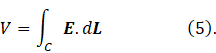
According to equation 1 of post 25.13, the induced voltage is given by
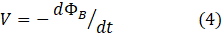
where ΦB is the magnetic flux. This equation describes the induced voltage when a conducting loop experiences a change in magnetic field. The work done in moving charge, q, around this loop is

as explained in post 17.44. If F is the force required to move these charges and δL represents an infinitesimal segment of the loop (both in magnitude and direction), then the work done can also be written as the line integral
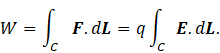
The second step comes from the definition of an electric field. Here C at the foot of the integral sign denotes integration around the loop. Equating these two expressions for W gives
In post 25.12, I expressed the magnetic flux as
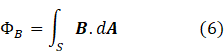
that is an integral over an entire surface with respect to the surface area A; A is a vector because its orientation can be represented by a unit vector perpendicular to its surface. The S at the foot of the integral sign denotes integration over the whole surface.
Substituting equations 5 and 6 into equation 4 gives
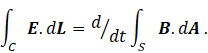
Next, we apply Stokes’ theorem (appendix 2) to this equation, giving the result
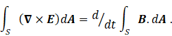
From which it follows that
The final step assumes no change in the geometry of the surface.
Appendix 2. Stokes’ theorem
In post 25.12, we met Gauss’s divergence theorem which states that, for a vector field F
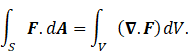
Be careful: in this appendix, F denotes any vector field – in the main post it represents a force. This theorem relates a surface integral to a line integral.
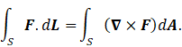
Stokes’ theorem relates a surface integral to a volume integral. It states that
The proof of this theorem is very tedious and I have no insights to offer on it. So, for more details, I refer you to a document named “The Integral Theorems” at https://www.damtp.cam.ac.uk/user/tong/vc/vc4.pdf
Which is part of an excellent source of information on vector calculus at https://www.damtp.cam.ac.uk/user/tong/vc/vc.pdf
