In post 25.10, I used a special case of the Biot-Savart law to define magnetic field. This law is named after the French physicists Jean-Baptiste Biot (1774-1862) and Félix Savart (1791-1841). But in post 25.15, I described how magnets were known long before Biot and Savart were born. Since magnets attract ferromagnetic material, they must exert a force and by definition are the source of a magnetic field. In this post, I want to explain how the original idea of a magnet relates to the definition I have given for a magnetic field and to explore the Biot-Savart law further.

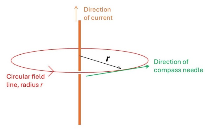
The picture above shows a circle of radius r whose centre is defined by a very long straight wire conducting an electrical current I; the wire is perpendicular to the plane of the circle. If we place a compass anywhere around this circle it will point along a tangent, as shown by the green arrow in the picture. This shows that there is a magnetic field surrounding the wire, as explained in post 25.15. This magnetic field only exists when the current if flowing. Since current is the flow of charge, the magnetic field exists only when charges are moving; stationary charges are associated with an electric field but not with a magnetic field.

The force that the field exerts on a sample of ferromagnetic material is a measure of its strength. Experiments show that the modulus, B, of the field is constant around a circle. So, at a distance r from the centre of the circle, the magnetic field line is a circle of radius r. Further experiments show that the field is proportional to I (doubling the current doubles B) and inversely proportional to r (doubling r decreases the B to a halfof its former value). We can express these results by the equation

where k is a constant. It is conventional to define a constant μ by

where μ is called the permeability of the stuff surrounding the wire. If the wire is surrounded by a vacuum, μ is denoted by μ_o and is called the permeability of free space; its value is 4π × 10^-7 T.m.A^-1; remember that the unit of B is the tesla (T). Now B is defined as

I discuss the definition of μ in more detail in appendix 1.

Remembering that the magnetic field is a force field and, hence, a vector, we represent it as B. What is the direction associated with B? It is given by the direction that the compass needle (green arrow) points in the picture above (see post 25.15). Now let’s consider a point P, in the picture below, whose position vector is r.

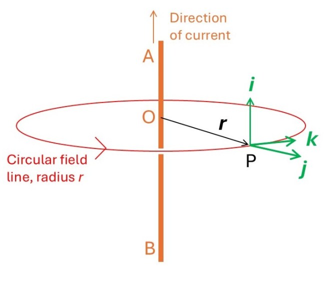
If we define unit vectors i in the direction the current flows and j in the direction of r, the compass needle then shows that B in involves the cross-product of i and j and is given by

This equation is given, without explanation, in post 25.10 but is more commonly written as

However this equation is written, it is a statement of the Biot-Savart law for an infinitely long, straight wire.

How can we calculate B if the wire is not straight? We consider an infinitesimal length, δL, of wire, where the direction of δL is the direction in which the current flows. Then a more general statement of the Biot-Savart law is that the infinitesimal field, at a point P, due to the current in our infinitesimal length of wire, is

Here ρ is a vector giving the position of P relative to δL. In appendix 2, I show that equation 4 is a special case of equation 6.

In principle, we can calculate B for any shape of wire by adding together the infinitesimal contributions from all its infinitesimal parts – that is by the mathematical operation of integration. In appendix 3, I do this at the centre of a flat coil. Most applications are mathematically more difficult and may require numerical integration.

Related posts

25.15 Magnets
25.10 Magnetic field
25.9 More about fields

Appendix 1

The appearance of 2π in the definition of μ.

Why do we define B using equation 3 and not equation 1? We could use equation 1 if we wanted to – this is the way I was taught electromagnetism. But I have chosen to use what is called the rationalised system in which we define μ by equation 2 and measure B in tesla.

I did something similar in post 25.9 where I defined permittivity, ε, and the electric field, E, at a point P at a vector separation r from a charge q by

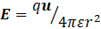
where u is a unit vector in the direction of r. So I could have written this definition as

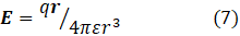
Comparing equations 3 and 7, you will see that a factor of 2π has been introduced in an equation describing a system with cylindrical symmetry and a factor of 4π for a system with spherical symmetry.

You might also notice that a factor of 4π appears in equation 6 where B has spherical symmetry because it is the field about a point (an elemental length) and so has spherical symmetry.

Writing these definitions in a way that depends on the symmetry of a field is the essential feature of the rationalised system of units. Why do we use rationalised units? The reason is to stop a factor of 4π appearing, apparently at random, in some of Maxwell’s equations.

Appendix 2

Derivation of equation 1 from Equation 2.

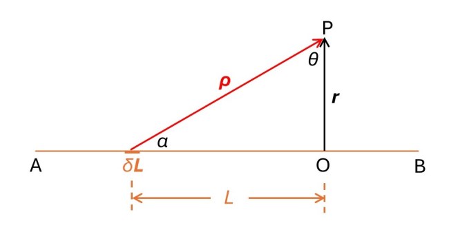
In the picture above, A and B are points on an infinitely long conducting wire in which a current, I, flows, in the direction from B to A. O is a point on the wire defined to be an origin. P is a point whose position is given by the vector r, perpendicular to the wire.

I am going to start by calculating the infinitesimal magnetic field at P arising from the current flowing in an element of wire described by the vector δL, whose position is given by the vector L that points from A to B. I define ρ as the vector position of P relative to the position of δL. Then the infinitesimal magnetic field is given by equation 5. From the definition of the cross product of vectors, this becomes

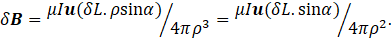
where u is a unit vector perpendicular to the plane of the picture and pointing away from you. Here α is the angle between ρ and the wire.

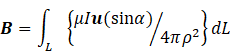
where the L, at the foot of the integral sign, denotes integration along the total length of the infinite wire. This integral is a mess because α and ρ are not independent. To keep the equations simple, I am going to define the angle θ by

The picture shows that θ is the internal angle at P of the right-angled triangle formed by r, ρ and the wire.

so that our integral becomes

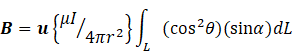
taking all the constants from out of the integral sign. From the definition of θ,   sinα = cosθ   (see post 16.50), so that our integral now becomes

Now notice, from the definition of the tangent of an angle, that

so that

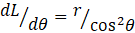
see post 22.10. We can nowrewrite our integral as

which is identical to equation 4 when we note that u is perpendicular to i and j. The limits of integration, in the equation above, arise because   90^o < θ ≤ 180^o   defines the length of the infinite wire.

Appendix 3

B at the centre of a flat coil.

A flat coil consists of a single length of insulated wire bent circles with the same radius that share the same centre; each circle is a loop of the coil. In the picture below, a current, I, flows in an anti-clockwise direction around a coil of radius ρ. I am going to consider the magnetic field at P, the centre of the coil, caused by the current flowing in an elemental arc of length, δL, of a single loop of wire; the direction of a vector δL is the same as the direction of the current.

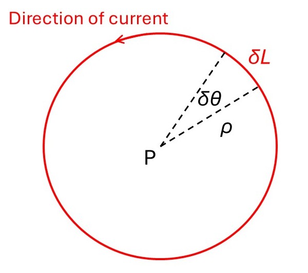
According to equation 6, this field is

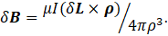
If the arc subtends an elemental angle, δθ, at P,   δL = ρ.δθ   , so that δL is given by u(ρ.δθ), where u is a unit vector in the direction of δL. Now we can write

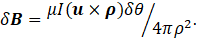
From the definition of the cross product of vectors   u × ρ   is always ρn, where n is a unit vector pointing towards you from the plane of the picture, so that

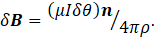
So that the total field at the current of the coil is given by integrating this result along the total length of the of the wire, that is by the definition integral

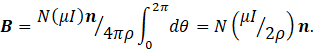
where N is the number of circular loops in the coil.